Fit Analyses

Linear Models

SAS/INSIGHT fit analysis provides the traditional parametric regression analysis assuming that the regression function is linear in the unknown parameters. The relationship is expressed as an equation that predicts a response variable from a linear function of explanatory variables. Besides the usual estimators and test statistics produced for a regression, a fit analysis can produce many diagnostic statistics. Collinearity diagnostics measure the strength of the linear relationship among explanatory variables and how this affects the stability of the estimates. Influence diagnostics measure how each individual observation contributes to determining the parameter estimates and the fitted values. In matrix algebra notation, a linear model is written as

$y = X {\beta} + {{\epsilon}}$

where y is the n×1 vector of responses, X is the n×p design matrix (rows are observations and columns are explanatory variables), $\beta$ is the p×1 vector of unknown parameters, and ${\epsilon}$ is the n×1 vector of unknown errors. Each effect in the model generates one or more columns in a design matrix X. The first column of X is usually a vector of 1's used to estimate the intercept term. In general, no-intercept models should be fit only when theoretical justification exists. Refer to the chapter on the GLM procedure in the SAS/STAT User's Guide for a description of the model parameterization. The classical theory of linear models is based on some strict assumptions. Ideally, the response is measured with all the explanatory variables controlled in an experimentally determined environment. If the explanatory variables do not have experimentally fixed values but are stochastic, the conditional distribution of y given X must be normal in the appropriate form.

Less restrictive assumptions are as follows:

The form of the model is correct (all important X variables have been included).
Explanatory variables are measured without error.
The expected value of the errors is 0.
The variance of the errors (and thus the response variable) is constant across observations (denoted by ${\sigma}^2$ ).
The errors are uncorrelated across observations.

If all the necessary assumptions are met, the least-squares estimates of $\beta$ are the best linear unbiased estimates (BLUE); in other words, the estimates have minimum variance among the class of estimators that are unbiased and are linear functions of the responses. In addition, when the error term is assumed to be normally distributed, sampling distributions for the computed statistics can be derived. These sampling distributions form the basis for hypothesis tests on the parameters. The method used to estimate the parameters is to minimize the sum of squares of the differences between the actual response values and the values predicted by the model. An estimator b for $\beta$ is generated by solving the resulting normal equations

(X'X)b = X'y

yielding

b = (X'X)^-1 X'y

Let H be the projection matrix for the space spanned by X, sometimes called the hat matrix,

H = X (X'X)^-1 X'

Then the predicted mean vector of the n observation responses is

$\hat{y} = X{b} = H y$

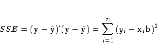
The sum of squares for error is

$SSE = {(y-\hat{y})'} (y-\hat{y}) = \sum_{i=1}^n{( y_{i} - x_{i}b)^2}$

where x_i is the ith row of the X matrix. Assume that X is of full rank. The variance ${\sigma}^2$ of the error is estimated by the mean square error

s² = MSE = [SSE/(n - p)]

The parameter estimates are unbiased:

${E(b) = {\beta}}$

${E( s^2) = {\sigma}^2}.$

The covariance matrix of the estimates is

$\rm{Var}(b) = ({X'}X)^{-1} {\sigma}^2$

The estimate of the covariance matrix, ${\hat{\rm{Var}}(b)}$ , is obtained by replacing ${\sigma}^2$ with its estimate, s², in the preceding formula:

$\hat{\rm{Var}}(b) = ({X'}X)^{-1} s^2$

The correlations of the estimates,

S^-1/2 (X'X)^-1 S^-1/2

are derived by scaling to one on the diagonal, where S = diag ( (X'X)^-1). If the model is not full rank, the matrix X'X is singular. A generalized (g2) inverse (Pringle and Raynor 1971), denoted as (X'X)^-, is then used to solve the normal equations, as follows:

b = (X'X)^- X'Y

However, this solution is not unique, and there are an infinite number of solutions using different generalized inverses. In SAS/INSIGHT software, the fit analysis chooses a basis of all variables that are linearly independent of previous variables and a zero solution for the remaining variables.

Related
Reading Multiple Regression, Chapter 14.

Related
Reading Analysis of Variance, Chapter 15.

Chapter Contents
Previous
Next
Top