Methods for Estimating the Standard Deviation

XCHART Statement

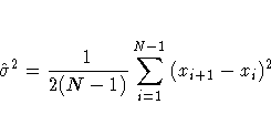
Methods for Estimating the Standard Deviation

It is recommended practice to provide a stable estimate or standard value for $\sigma$ with either the SIGMA0= option or the variable _STDDEV_ in a LIMITS= data set. However, if such a value is not available, you can compute an estimate $\hat{\sigma}$ from the data, as described in this section.

This section provides formulas for various methods used to estimate the standard deviation $\sigma$ . One method is applicable with individual measurements, and three are applicable with subgrouped data. The methods can be requested with the SMETHOD= option.

Method for Individual Measurements

When the cumulative sums are calculated from individual observations

x₁,x₂, ... ,x_N

rather than subgroup samples of two or more observations, the CUSUM procedure estimates $\sigma$ as $\sqrt{\hat{\sigma}^2}$ ,where

$\hat{\sigma}^2=\frac{1}{2(N-1)} \sum_{i=1}^{N-1}{(x_{i+1}-x_{i})^2}$

where N is the number of observations. Wetherill (1977) states that the estimate of the variance is biased if the measurements are autocorrelated.

Note that you can compute alternative estimates (for instance, robust estimates or estimates based on variance components models) by analyzing the data with SAS modeling procedures or your own DATA step program. Such estimates can be passed to the CUSUM procedure as values of the variable _STDDEV_ in a LIMITS= data set.

NOWEIGHT Method for Subgroup Samples

This method is the default for cusum charts for subgrouped data. The estimate is

$\hat{\sigma}=\frac{(s_{1}/c_{4}(n_{1}))+ ... + (s_{N}/c_{4}(n_{N}))}N$

where n_i is the sample size of the i^th subgroup, N is the number of subgroups for which $n_{i}\geq2$ , s_i is the sample standard deviation of the observations x_i1, ... ,x_{in_i} in the i^th subgroup.

$s_{i}=\sqrt{(1/(n_{i}-1))\textstyle \sum_{j=1}^{n_{i}}{(x_{ij}-\bar{X}_{i})^2 } }$

and

$c_{4}(n_{i})=\frac{\Gamma(n_{i}/2)\sqrt{2/(n_{i}-1)} } {\Gamma((n_{i}-1)/2)}$

where $\Gamma(\cdot)$ denotes the gamma function, and $\bar{X}_{i}$ denotes the i^th subgroup mean. A subgroup standard deviation s_i is included in the calculation only if $n_{i}\geq2$ . If the observations are normally distributed, then the expected value of s_i is

$E(s_{i})=c_{4}(n_{i})\sigma$

Thus, $\hat{\sigma}$ is the unweighted average of N unbiased estimates of $\sigma$ . This method is described in the ASTM Manual on Presentation of Data and Control Chart Analysis.

MVLUE Method for Subgroup Samples

If you specify SMETHOD=MVLUE, a minimum variance linear unbiased estimate (MVLUE) is computed, as introduced by Burr (1969, 1976). This estimate is a weighted average of unbiased estimates of $\sigma$ of the form

s_i/c₄(n_i)

where

s_i is the standard deviation of the i^th subgroup.

c₄(n_i) is the unbiasing factor defined previously.

n_i is the i^th subgroup sample size, i = 1,2, ... ,N.

N is the number of subgroups for which $n_{i}\geq2$ .

The estimate is

$\hat{\sigma}=\frac{h_{1}s_{1}/c_{4}(n_{1})+ ... + h_{N}s_{N}/c_{4}(n_{N})}{h_{1}+ ... +h_{N}}$

where h_i = c²₄(n_i)/(1-c²₄(n_i)) . A subgroup standard deviation s_i is included in the calculation only if $n_{i}\geq2$ .

The MVLUE assigns greater weight to estimates of $\sigma$ from subgroups with larger sample sizes and is intended for situations where the subgroup sample sizes vary. If the subgroup sample sizes are constant, the MVLUE reduces to the default estimate (NOWEIGHT).

RMSDF Method for Subgroup Samples

If you specify SMETHOD=RMSDF, a weighted root-mean-square estimate is computed:

$\hat{\sigma}=\frac { \sqrt{(n_{1}-1)s^2_{1}+ ... +(n_{N}-1)s^2_{N}} } {c_{4}(n)\sqrt{n_{1}+ ... +n_{N}-N} }$

where

n_i is the sample size of the i^th subgroup.

N is the number of subgroups for which $n_{i}\geq2$ .

s_i is the sample standard deviation of the i^th subgroup.

c₄(n_i) is the unbiasing factor defined previously.

n is equal to (n₁+ ... +n_N)-(N-1) .

The weights in the root-mean-square expression are the degrees of freedom n_i-1. A subgroup standard deviation s_i is included in the calculation only if $n_{i}\geq2$ .

If the unknown standard deviation $\sigma$ is constant across subgroups, the root-mean-square estimate is more efficient than the minimum variance linear unbiased estimate. However, as noted by Burr (1969), "the constancy of $\sigma$ is the very thing under test," and if $\sigma$ varies across subgroups, the root-mean-square estimate tends to be more inflated than the MVLUE.

Chapter Contents
Previous
Next
Top

s_i	is the standard deviation of the i^th subgroup.
c₄(n_i)	is the unbiasing factor defined previously.
n_i	is the i^th subgroup sample size, i = 1,2, ... ,N.
N	is the number of subgroups for which $n_{i}\geq2$ .

n_i	is the sample size of the i^th subgroup.
N	is the number of subgroups for which $n_{i}\geq2$ .
s_i	is the sample standard deviation of the i^th subgroup.
c₄(n_i)	is the unbiasing factor defined previously.
n	is equal to (n₁+ ... +n_N)-(N-1) .