Introduction to Structural Equations with Latent Variables

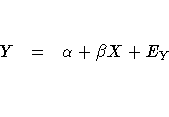
Specifying Structural Equation Models

Consider fitting a linear equation to two observed variables, Y and X. Simple linear regression uses the model of a particular form, labeled for purposes of discussion, as Model Form A.

Model Form A

$Y & = & \alpha + \beta X + E_Y \$

where $\alpha$ and $\beta$ are coefficients to be estimated and E_Y is an error term. If the values of X are fixed, the values of E_Y are assumed to be independent and identically distributed realizations of a normally distributed random variable with mean zero and variance Var(E_Y). If X is a random variable, X and E_Y are assumed to have a bivariate normal distribution with zero correlation and variances Var(X) and Var(E_Y), respectively. Under either set of assumptions, the usual formulas hold for the estimates of the coefficients and their standard errors (see Chapter 3, "Introduction to Regression Procedures").

In the REG or SYSLIN procedure, you would fit a simple linear regression model with a MODEL statement listing only the names of the manifest variables:

   proc reg;
      model y=x;
   run;

You can also fit this model with PROC CALIS, but you must explicitly specify the names of the parameters and the error terms (except for the intercept, which is assumed to be present in each equation). The linear equation is given in the LINEQS statement, and the error variance is specified in the STD statement.

   proc calis cov;
      lineqs y=beta x + ex;
      std ex=vex;
   run;

The parameters are the regression coefficient BETA and the variance VEX of the error term EX. You do not need to type an * between BETA and X to indicate the multiplication of the variable by the coefficient.

The LINEQS statement uses the convention that the names of error terms begin with the letter E, disturbances (errors terms for latent variables) in equations begin with D, and other latent variables begin with F for "factor." Names of variables in the input SAS data set can, of course, begin with any letter.

If you leave out the name of a coefficient, the value of the coefficient is assumed to be 1. If you leave out the name of a variance, the variance is assumed to be 0. So if you tried to write the model the same way you would in PROC REG, for example,

   proc calis cov;
      lineqs y=x;

you would be fitting a model that says Y is equal to X plus an intercept, with no error.

The COV option is used because PROC CALIS, like PROC FACTOR, analyzes the correlation matrix by default, yielding standardized regression coefficients. The COV option causes the covariance matrix to be analyzed, producing raw regression coefficients. See Chapter 3, "Introduction to Regression Procedures," for a discussion of the interpretation of raw and standardized regression coefficients.

Since the analysis of covariance structures is based on modeling the covariance matrix and the covariance matrix contains no information about means, PROC CALIS neglects the intercept parameter by default. To estimate the intercept, change the COV option to UCOV, which analyzes the uncorrected covariance matrix, and use the AUGMENT option, which adds a row and column for the intercept, called INTERCEP, to the matrix being analyzed. The model can then be specified as

   proc calis ucov augment;
      lineqs y=alpha intercep + beta x + ex;
      std ex=vex;
   run;

In the LINEQS statement, intercep represents a variable with a constant value of 1; hence, the coefficient alpha is the intercept parameter.

Other commonly used options in the PROC CALIS statement include

MODIFICATION to display model modification indices
RESIDUAL to display residual correlations or covariances
STDERR to display approximate standard errors
TOTEFF to display total effects

For ordinary unconstrained regression models, there is no reason to use PROC CALIS instead of PROC REG. But suppose that the observed variables Y and X are contaminated by error, and you want to estimate the linear relationship between their true, error-free scores. The model can be written in several forms. A model of Form B is as follows.

Model Form B

$Y & = & \alpha + \beta F_X + E_Y \ X & = & F_X + E_X \ {Cov}(F_X,E_X) & = & {Cov}(F_X,E_Y) = {Cov}(E_X,E_Y) = 0$

This model has two error terms, E_Y and E_X, as well as another latent variable F_X representing the true value corresponding to the manifest variable X. The true value corresponding to Y does not appear explicitly in this form of the model.

The assumption in Model Form B is that the error terms and the latent variable F_X are jointly uncorrelated is of critical importance. This assumption must be justified on substantive grounds such as the physical properties of the measurement process. If this assumption is violated, the estimators may be severely biased and inconsistent.

You can express Model Form B in PROC CALIS as follows:

   proc calis cov;
      lineqs y=beta fx + ey,
             x=fx + ex;
      std fx=vfx,
          ey=vey,
          ex=vex;
   run;

You must specify a variance for each of the latent variables in this model using the STD statement. You can specify either a name, in which case the variance is considered a parameter to be estimated, or a number, in which case the variance is constrained to equal that numeric value. In general, you must specify a variance for each latent exogenous variable in the model, including error and disturbance terms. The variance of a manifest exogenous variable is set equal to its sample variance by default. The variances of endogenous variables are predicted from the model and are not parameters. Covariances involving latent exogenous variables are assumed to be zero by default. Covariances between manifest exogenous variables are set equal to the sample covariances by default.

Fuller (1987, pp. 18 -19) analyzes a data set from Voss (1969) involving corn yields (Y) and available soil nitrogen (X) for which there is a prior estimate of the measurement error for soil nitrogen Var(E_X) of 57. You can fit Model Form B with this constraint using the following SAS statements.

   data corn(type=cov);
      input _type_ $ _name_ $ y x;
      datalines;
   n    . 11       11
   mean . 97.4545  70.6364
   cov  y 87.6727  .
   cov  x 104.8818 304.8545
   ;

   proc calis data=corn cov stderr;
      lineqs y=beta fx + ey,
             x=fx + ex;
      std ex=57,
          fx=vfx,
          ey=vey;
   run;

In the STD statement, the variance of EX is given as the constant value 57. PROC CALIS produces the following estimates.

The SAS System

The CALIS Procedure

Covariance Structure Analysis: Maximum Likelihood Estimation

y	=	0.4232	*	fx	+	1.0000	ey
Std Err		0.1658		beta
t Value		2.5520
x	=	1.0000		fx	+	1.0000	ex

Variances of Exogenous Variables
Variable	Parameter	Estimate	Standard Error	t Value
fx	vfx	247.85450	136.33508	1.82
ey	vey	43.29105	23.92488	1.81
ex		57.00000

Figure 14.1: Measurement Error Model for Corn Data

PROC CALIS also displays information about the initial estimates that can be useful if there are optimization problems. If there are no optimization problems, the initial estimates are usually not of interest; they are not be reproduced in the examples in this chapter.

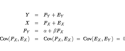
You can write an equivalent model (labeled here as Model Form C) using a latent variable F_Y to represent the true value corresponding to Y.

Model Form C

$Y & = & F_Y + E_Y \X & = & F_X + E_X \F_Y & = & \alpha + \beta F_X \{Cov}(F_X,E_X) & = & {Cov}(F_X,E_X) = {Cov}(E_X,E_Y) = 0$

The first two of the three equations express the observed variables in terms of a true score plus error; these equations are called the measurement model. The third equation, expressing the relationship between the latent true-score variables, is called the structural or causal model. The decomposition of a model into a measurement model and a structural model (Keesling 1972; Wiley 1973; J $\ddot{o}$ reskog 1973) has been popularized by the program LISREL (J $\ddot{o}$ reskog and S $\ddot{o}$ rbom 1988). The statements for fitting this model are

   proc calis cov;
      lineqs y=fy + ey,
             x=fx + ex,
             fy=beta fx;
      std fx=vfx,
          ey=vey,
          ex=vex;
   run;

You do not need to include the variance of F_Y in the STD statement because the variance of F_Y is determined by the structural model in terms of the variance of F_X, that is, Var(F_Y)= $\beta^2$ Var(F_X).

Correlations involving endogenous variables are derived from the model. For example, the structural equation in Model Form C implies that F_Y and F_X are correlated unless $\beta$ is zero. In all of the models discussed so far, the latent exogenous variables are assumed to be jointly uncorrelated. For example, in Model Form C, E_Y, E_X, and F_X are assumed to be uncorrelated. If you want to specify a model in which E_Y and E_X, say, are correlated, you can use the COV statement to specify the numeric value of the covariance Cov(E_Y, E_X) between E_Y and E_X, or you can specify a name to make the covariance a parameter to be estimated. For example,

   proc calis cov;
      lineqs y=fy + ey,
             x=fx + ex,
             fy=beta fx;
      std fy=vfy,
          fx=vfx,
          ey=vey,
          ex=vex;
      cov ey ex=ceyex;
   run;

This COV statement specifies that the covariance between EY and EX is a parameter named CEYEX. All covariances that are not listed in the COV statement and that are not determined by the model are assumed to be zero. If the model contained two or more manifest exogenous variables, their covariances would be set to the observed sample values by default.

Identification of Models

Chapter Contents
Previous
Next
Top