What's New in SAS Software

SAS/INSIGHT Software

Surface Plots

Surface plots are three-dimensional displays of continuous response surfaces on the regular grids of the explanatory variables.

When there are two explanatory variables in the model, a parametric response surface plot is created by default. You can also generate a nonparametric kernel or thin-plate smoothing spline response surface plot. With more than two explanatory variables in the model, a parametric profile of response surface plot with the first two explanatory variables can be created. The values of the remaining explanatory variables are set to their corresponding means in the plot. You can use sliders to change the values of the remaining explanatory variables.

Parametric Surface Plot

With two explanatory interval variables in the model, a parametric surface plot is a continuous surface plot of the predicted responses from the fitted parametric model on a set of regular grids of the explanatory variables.

Smoothing Spline Surface Plot

Two criteria can be used to select an estimator ${\hat{ f_{{\lambda}}}}$ for the function f:

goodness of fit to the data
smoothness of the fit

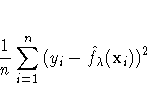
A standard measure of goodness of fit is the mean residual sum of squares

$\hspace*{0.2in} \frac{1}n\sum_{i=1}^n{( y_{i}- \hat{ f_{{\lambda}}}( x_{i}))^2}$

A measure of the smoothness of a fit is an integrated squared second derivative

$J_{2} ( f_{{\lambda}}) = \int_{-{\infty}}^{{\infty}}{\int_{-{\infty}}^{{\infty}... ...artial}^2 f_{{\lambda}}}{{\partial} x_{2}^2 } )^2 \, d x_{1} } \, d x_{2} }$

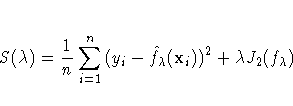
A single criterion that combines the two criteria is then given by

$\hspace*{0.2in} S({\lambda}) = \frac{1}n \sum_{i=1}^n{( y_{i}- \hat{ f_{{\lambda}}}( x_{i}))^2} + {\lambda} J_{2} ( f_{{\lambda}})$

where ${\hat{ f_{{\lambda}}}}$ belongs to the set of all continuously differentiable functions with square integrable second derivatives, and ${\lambda}$ is a positive constant.

The estimator that results from minimizing S( ${\lambda}$ )is called a thin-plate smoothing spline estimator. Wahba and Wendelberger (1980) derived a closed form expression for the thin-plate smoothing spline estimator.

Note: The computations for a thin-plate smoothing spline is time-intensive, especially for large data sets.

The smoothing parameter ${\lambda}$ controls the amount of smoothing; that is, it controls the trade-off between the goodness of fit to the data and the smoothness of the fit. You select a smoothing parameter ${\lambda}$ by specifying a constant c in the formula

$\hspace*{0.2in} {\lambda} = c / 100$

The values of the explanatory variables are scaled by their corresponding interquartile ranges before the computations. This makes the computations independent of the units of X₁ and X₂.

After choosing Graphs:Surface Plot:Spline from the menu, you specify a smoothing parameter selection method in the Spline Fit dialog.

The default Method:GCV uses a c value that minimizes the generalized cross-validation mean squared error ${ \rm{MSE}_{GCV}({\lambda})}$ .

Kernel Surface Plot

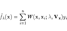
A kernel estimator uses an explicitly defined set of weights at each point x to produce the estimate at x. The kernel estimator of f has the form

$\hspace*{0.2in} \hat{ f_{{\lambda}}}(x) = \sum_{i=1}^n{W( x , x_{i}; {\lambda}, V_{x}) y_{i}}$

where W ${( x , x_{i}; {\lambda}, V_{x})}$ is the weight function that depends on the smoothing parameter ${\lambda}$ and the diagonal matrix V_x of sample interquartile ranges.

The weights are derived from a single function that is independent of the design

$\hspace*{0.2in} W( x , x_{i}; {\lambda}, V_{x}) = \frac{K_{0} ( (x - x_{i})/{\lambda}, V_{x} )}{\sum_{j=1}^n{K_{0} ( (x - x_{j})/{\lambda}, V_{x} ) } }$

where K₀ is a kernel function and ${\lambda}$ is the bandwidth or smoothing parameter. The weights are nonnegative and sum to 1.

Symmetric probability density functions commonly used as kernel functions are

Normal, $K_{0}(t, V) = \frac{1}{2\pi} \exp( - \frac{1}2 {t'} V^{-1} t) \hspace*{0.4in} \rm{forall}t$
Quadratic, $K_{0}(t, V) = \{ \frac{2}{\pi} (1-t' V^{-1} t) & \hspace*{0.3in} \rm{for} t' V^{-1} t \le 1,\\ 0 & \hspace*{0.3in} \rm{otherwise} .$
Biweight, $K_{0}(t, V) = \{ \frac{3}{{\pi}} (1-{t'} V^{-1} t)^2 & \hspace*{0.3in} \rm{for} {t'} V^{-1} t {\le} 1,\\ 0 & \hspace*{0.3in} \rm{otherwise} .$
Triweight, $K_{0}(t, V) = \{ \frac{4}{{\pi}} (1-{t'} V^{-1} t)^3 & \hspace*{0.3in} \rm{for} {t'} V^{-1} t {\le} 1,\\ 0 & \hspace*{0.3in} \rm{otherwise} .$

You select a bandwidth ${\lambda}$ for each kernel estimator by specifying c in the formula

${\lambda} = n^{-\frac{1}6} c$

where n is the sample size. Both ${\lambda}$ and c are independent of the units of X.

SAS/INSIGHT software divides the range of each explanatory variable into a number of evenly spaced intervals, then estimate the kernel fit on this grid. For a data point x_i that lies between two grid points, a linear interpolation is used to compute the predicted value. For x_i that lies inside a square of grid points, a pair of points that on the same vertical line as x_i and each lies between two grid points can be found. A linear interpolation of these two points is used to compute the predicted value.

After choosing Graphs:Surface Plot:Kernel from the menu, you specify a kernel and smoothing parameter selection method in the Kernel Fit dialog.

By default, SAS/INSIGHT software divides the range of each explanatory variable into 20 evenly spaced intervals, uses a normal weight, and uses a c value that minimizes ${ \rm{MSE}_{GCV}({\lambda})}$ .

Parametric Profile Surface Plot

With more than two explanatory interval variables in the model, a parametric profile surface plot is a continuous surface plot of the predicted responses from the fitted parametric model on a set of regular grids of a pair of explanatory variables. The values of the remaining explanatory variables are initially set at their means and can be adjusted with the sliders.

By default, the first two explanatory variables are used in the surface plot. You can also create profile surface plots for other explanatory variables by selecting the two variables before choosing Graphs:Surface Plot:Parametric profile.

Chapter Contents
Previous
Next
Top