No Title

Stat 330 Assignment 10 Partial Solutions

Chapter 12 Q2: When the accelerated strength is x the regression model says that 28 day strength is normally distributed with SD 350 and mean .

For x=2000 the mean becomes 4400. The probability that 28 day strength is more than 5000 is the probability that a standard normal variate is more than (5000-4400)/350=1.71. This probability is 0.0436.

For x=2500 the mean is 5050 and the probability is the area to the right of -50/350 which is 0.556.

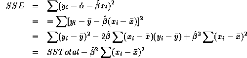
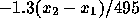
Let be the observation at x=2500 and the observation x=2000. Then the mean of is 1.3(500)=650 while the SD of the difference is . The probability we want is that a standard normal is more than (1000-650)/495=0.707.This is roughly 0.24.

Now is normal with mean and SD 495. We want the probability that or the probability to the right of to be 0.95. This means that 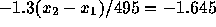or . The answer is then 626.

Q16: I used the following SAS code and ran the code twice with and without the last point.
options pagesize =60 linesize=80; data q16; infile 'q16.dat'; input x y; proc reg; model y=x; plot residual.*predicted.; plot y*x; run;
The output for the full data set is
Dependent Variable: Y Analysis of Variance Sum of Mean Source DF Squares Square F Value Prob>F Model 1 538208.57051 538208.57051 385.024 0.0001 Error 4 5591.42949 1397.85737 C Total 5 543800.00000 Root MSE 37.38793 R-square 0.9897 Dep Mean 560.00000 Adj R-sq 0.9871 C.V. 6.67642 Parameter Estimates Parameter Standard T for H0: Variable DF Estimate Error Parameter=0 Prob > |T| INTERCEP 1 137.875631 26.37756553 5.227 0.0064 X 1 9.311567 0.47454663 19.622 0.0001 ----+-----+-----+-----+-----+-----+-----+-----+-----+-----+-----+---- RESIDUAL | | | | 50 + + | | | | | 1 | | | 40 + + | | | | | | | | 30 + + | | | | | | | | 20 + 1 + | | | | | | R | 1 | e 10 + + s | | i | | d | 1 | u | | a 0 + + l | | | | | | | | -10 + + | | | | | | | | -20 + + | | | | | | | | -30 + + | | | | | | | 1 | -40 + 1 + | | | | ----+-----+-----+-----+-----+-----+-----+-----+-----+-----+-----+---- 200 300 400 500 600 700 800 900 1000 1100 1200 Predicted Value of Y PRED ----+-----+-----+-----+-----+-----+-----+-----+-----+-----+-----+-----+---- Y | | | | | | | | | | 1200 + 1 + | | | | | | 1100 + + | | | | | | 1000 + + | | | | | | 900 + + | | | | | | 800 + + | | | | | | 700 + + | | | | | | 600 + + | | | 1 | | | 500 + 1 + | 1 | | | | | 400 + + | | | 1 | | | 300 + + | 1 | | | | | 200 + + | | | | | | | | ----+-----+-----+-----+-----+-----+-----+-----+-----+-----+-----+-----+---- 10 20 30 40 50 60 70 80 90 100 110 120 X
while that for the edited data set is
Sum of Mean Source DF Squares Square F Value Prob>F Model 1 49839.81693 49839.81693 61.274 0.0043 Error 3 2440.18307 813.39436 C Total 4 52280.00000 Root MSE 28.52007 R-square 0.9533 Dep Mean 432.00000 Adj R-sq 0.9378 C.V. 6.60187 Parameter Estimates Parameter Standard T for H0: Variable DF Estimate Error Parameter=0 Prob > |T| INTERCEP 1 190.352403 33.40167361 5.699 0.0107 X 1 7.551487 0.96470574 7.828 0.0043 -+----+----+----+----+----+----+----+----+----+----+----+----+----+-- RESIDUAL | | | | | | | | 30 + 1 + | | | | | | | 1 | | | | | 20 + + | | | | | | | | | | | | 10 + + | | | | R | | e | | s | | i | | d 0 + + u | | a | | l | | | | | | | | -10 + + | | | | | | | 1 1 | | | | | -20 + + | | | 1 | | | | | | | | | -30 + + | | | | | | -+----+----+----+----+----+----+----+----+----+----+----+----+----+-- 280 300 320 340 360 380 400 420 440 460 480 500 520 540 Predicted Value of Y PRED -----+----+----+----+----+----+----+----+----+----+----+----+----+----+----- 600 + + | | | | | | | | | | | 1 | 550 + + | | | | | | | | | | | | 500 + 1 + | | | | Y | | | 1 | | | | | 450 + + | | | | | | | | | | | | 400 + + | | | | | | | | | | | | 350 + 1 + | | | | | | | | | | | | 300 + + | | | | | 1 | | | | | | | 250 + + -----+----+----+----+----+----+----+----+----+----+----+----+----+----+----- 12.5 15.0 17.5 20.0 22.5 25.0 27.5 30.0 32.5 35.0 37.5 40.0 42.5 45.0 X

The scatter plot for the full data set seems reasonable.

The regression equation is .

This just asks for but I doubt the utility of the calculation unless the x levels were set by random sampling of pairs. The value is 0.99.

There are many ways to compare the two lines. One is based on examining the difference in fitted slopes: 9.31 compared to 7.55 with a standard error of either about 0.47 or 1. This is not actually a significant difference assuming the model holds. Another approach is suggested in the text. The predicted value of Y when x is 112 is, for the second line 7.55(112)+190.4 or about 1036. The standard deviation of is given on page 503 and you could carry out a t-test using 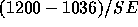and getting P-values from the t-distribution on 3 degrees of freedom.

Q18: You are asked to veryify that . The right hand side is which is evidently .

Q28: The edited sas output is
Sum of Mean Source DF Squares Square F Value Prob>F Model 1 8.17906 8.17906 674.982 0.0001 Error 8 0.09694 0.01212 C Total 9 8.27600 Root MSE 0.11008 R-square 0.9883 Dep Mean 3.92000 Adj R-sq 0.9868 C.V. 2.80814 Parameter Estimates Parameter Standard T for H0: Variable DF Estimate Error Parameter=0 Prob > |T| INTERCEP 1 2.141648 0.07679262 27.889 0.0001 X 1 0.006801 0.00026176 25.980 0.0001

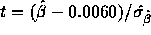The output gives the estimated standard error of the slope as 0.077 and the square root of the mean squared error as 0.11.

The test is based on which is 3.06. You get a P-value from t tables on 8 degrees of freedom and conclude that the slope is not 0.0060 ( two tailed).

Q32: We have (in my notation). You are allowed to assume that . Now
Putting the two pieces we get 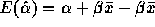which is just .

Q34: Let and . The fitted slope based on the starred data is
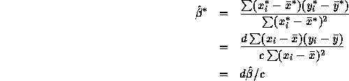
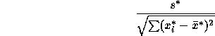
The estimated standard error of is
To evaluate this note first that 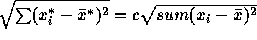. Next
Assembling the pieces shows that

Q52:

The test statistic is on 12 degrees of freedom. For a two sided test I get P a bit over 0.10 and conclude that there is only quite weak evidence fo a correlation between content and gas porosity.

The percent variance explained is %.

Q56: Since P is less than 0.001 we would reject the null at the level 0.001 and conclude that the correlation is not 0. However, with such a large n it takes only a quite small correlation to produce a P value of 0.00032. (To be precise: the estimated value of must be either 0.16 or -0.16 which is a pretty weak correlation.)

Q58: The edited SAS output is
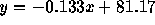
Sum of Mean Source DF Squares Square F Value Prob>F Model 1 25.62223 25.62223 17.604 0.0057 Error 6 8.73277 1.45546 C Total 7 34.35500 Root MSE 1.20643 R-square 0.7458 Dep Mean 77.72500 Adj R-sq 0.7034 C.V. 1.55217 Parameter Estimates Parameter Standard T for H0: Variable DF Estimate Error Parameter=0 Prob > |T| INTERCEP 1 81.173057 0.92589886 87.669 0.0001 X 1 -0.133258 0.03176040 -4.196 0.0057

The fitted line is .

This question asks you to test the hypothesis that the true slope is 0. The P value is 0.0057 from the output so that the hypothesis of no relation between x and Y is rejected.

The standard error of is inversely proportional to . Putting 4 data points at 0 and 4 at 50 makes equal to 5000 while the value for the data set is only about 1450. Thus the new design estimates more precisely. Using only 3 points at 0 and at 50 gives a sum of 3750 which is still much more precise than the design used.

You are supposed to plug 25 into the regression equation and then use the formulas on page 503 to attach a standard error to this number. You get 77.85 with an estimated standard error of 0.428. This does not really answer the question about whether or not efficiency has been precisely estimated but that seems to be something of a judgement.

Q62: I used SAS to get
General Linear Models Procedure R-Square C.V. Root MSE Y Mean 0.070002 26.22198 198.15080 755.66667 T for H0: Pr > |T| Std Error of Parameter Estimate Parameter=0 Estimate INTERCEPT 684.4057037 5.78 0.0007 118.3236387 X 14.8804795 0.73 0.4915 20.5000646
The test statistic is 0.73 with 7 degrees of freedom. Since the test is one sided we get a P value of 0.4915/2 which is certainly not significant. Thus it seems quite possible that there is no (linear) relation between eye weight and thickness.

Q67:

Since it clearly suffices to check that . But this last value is
as required.

You need to compute r and that's the answer except that if r is negative then for each SD below average on x you predict that r times that many SD's above average on y while the deviations are in the same direction if r is positive.

Q68: I begin with
Divide through by SSTotal and use the formula where , etc., to get
Then
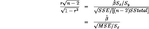
which is the usual t-statistic. Note the use of the fact that .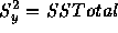

About this document ...

Next: About this document

Richard Lockhart
Mon Dec 2 12:25:22 PST 1996