STAT 330: 95-3

Assignment 5 Solutions

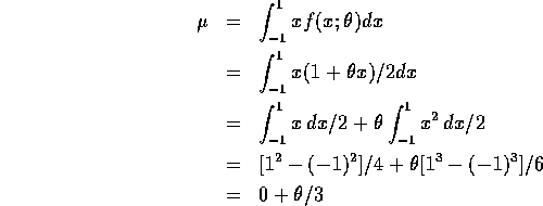
1. Chapter 6 Q 13: Let be the population mean. Then so we must evaluate . The definition is

   

   so that .

2. Chapter 6 Q 15: The moment of order r is which is given by

   

   Make the substitution for which and get

   

   For the special case r=2 we get the formula in the book (using ).

   1. According to the fact so that . Thus is unbiased.

   2. You square these numbers, add then divide by 20 and get 74.505 as in the appendix.

3. Chapter 6 Q 28:
   1. The log of the density is so that the log likelihood is

      

      To maximize this we take the derivative with respect to and set the result equal to 0 getting

      

      which has root which is the same as the unbiased estimate above.

   2. The median, m, of the distribution satisfies

      

      The integral may be done by substituting to get

      

      Solve this to get and then the mle of m is

      

4. Chapter 8 Q 26b: We are given so that the test rejects when t exceeds the t critical value on 7 degrees of freedom. The nearest curve in Table A.13 is for 6 degrees of freedom and the quantity d is For 6 df this appears to correspond to a of around 0.76 while for 9 df we would get about 0.65. My estimate is about a third of the way between them (because 7 is a third of the way between 6 and 9) or roughly .72.

5. Chapter 8 Q 30b: See the formula on page 319 and plug in to get

   

   so that n=24 would be needed. Notice that the formula for the sample size for a two sided level test is just the same as that\ for a one sided level test.

   It is also acceptable to do this using the t-test graphs as in the previous question. In fact, I think this is what the text intended really. If so you get a sample size of 19.

6. Chapter 9 Q 6 b,c: The rejection region of the test is

   

   which can be rewritten as

   

   The power function at is then the area to the right of the right hand side of this last formula under a standard normal curve. Plugging in numbers shows that we want the area to the left of which is .31. That is approximately. To get a probability of type II error equal to 0.1 we need

   

   Putting m=40 and plugging all the other numbers we get

   

   which leads to n of roughly 37 (actually a bit over so rounding up to 38 would be normal).

7. Chapter 9 Q 12: This is just the formula at the foot of page 351. We get

   

   which we round up to 50 for safety's sake.

8. Chapter 9 Q 73: This is a paired comparison problem. You take the differences, getting 3.2, -3.4, 0.4, 0.5, 0.3, -1.4, -0.3, 0, 3.5, -3.7, 3.7, 3.9, 1.6, 3.2. The one sample t statistic is 1.22 on 13 degrees of freedom leading to a 1 sided P value of 12% which is only weak evidence of higher TSI for the treatment than for the placebo.

• About this document ...