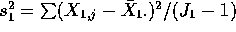
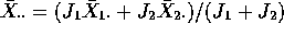
 be the population standard deviation
for control rats and
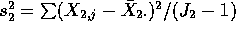
be the population standard deviation
for control rats and  be the treatment population standard
deviation. Then to test
be the treatment population standard
deviation. Then to test  against the one
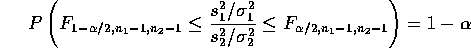
sided alternative
against the one
sided alternative  we compute
  and
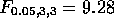
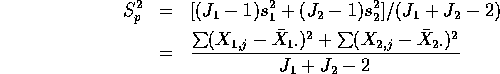
get upper tail P-values from F tables with 19 and 22 degrees of
freedom. We get
and
get upper tail P-values from F tables with 19 and 22 degrees of
freedom. We get  and P just a bit bigger than 0.01 so that we
conclude that the treatment population is more variable. (While the
question asks a one-tailed question it is not entirely clear to me that the
tail was not chosen after seeing the data; if so you should double the
P-value. The conclusion is not really changed.)
and P just a bit bigger than 0.01 so that we
conclude that the treatment population is more variable. (While the
question asks a one-tailed question it is not entirely clear to me that the
tail was not chosen after seeing the data; if so you should double the
P-value. The conclusion is not really changed.)
 has an F distribution so that
The right hand inequality holds if and only if

Similarly, the first inequality can be rearranged to be

so that the range between these two limits is a level  confidence
interval for
confidence
interval for  . For the data we have
 and
and  . The critical point
 while to find the lower tail critical point
we use
while to find the lower tail critical point
we use 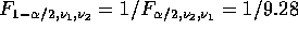 .
The interval is then
.
The interval is then 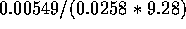 to
to  .
Note that some people may have put
.
Note that some people may have put  on top.
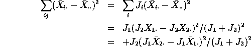
 . Use
. Use  and the fact that summing over
j just multiplies by J to get
and the fact that summing over
j just multiplies by J to get
 .
.
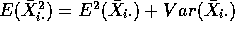 .
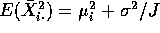
The variance of any average of J independent quantities each with
variance
.
The variance of any average of J independent quantities each with
variance  is just
  so we get
 .
.
 which, using (a) and the rule in (b) is
 .
.
 .
Expand out the square and use the fact that
.
Expand out the square and use the fact that 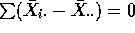 to see that
Take exepcted values and put in the results of (b) and (c) to get

 the second of these terms is 0 so
 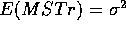 while under the alternative the second term is positive so that
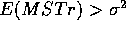 .
.
 we have
  ,
,  ,
and all the other
,
and all the other  so that the confidence interval for
 is
is 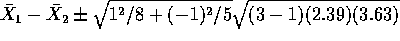 (where we use the level
  for a 95% confidence
interval). For the other intervals it is the values of the
for a 95% confidence
interval). For the other intervals it is the values of the  which
change. They are
which
change. They are  ,
,  and
and  respectively.
Only the contrast
respectively.
Only the contrast  is judged significantly different from 0.
(Note the use of
is judged significantly different from 0.
(Note the use of  not
not  ; these are 95% confidence
intervals.)
; these are 95% confidence
intervals.)
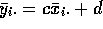 and
and 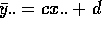 . Subtracting we get
 so the the SSE
for the y's is
so the the SSE
for the y's is  times the SSE for the x's. Similary we have
 so that the new SSTr is
  times the old SSTr.
The factors
times the old SSTr.
The factors  then cancel out in the formula for the F statistic so
that the new F statistic is exactly equal to the old F statistic.
then cancel out in the formula for the F statistic so
that the new F statistic is exactly equal to the old F statistic.
 for
for  and
and
 for
for  . The two sample variances are
 and
and
 .
Then the pooled estimate of
.
Then the pooled estimate of  is
is
which is just
which is in turn just the MSE.
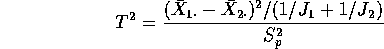
Now write 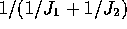 as
as 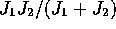 to see that
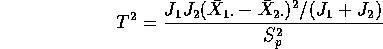
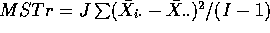
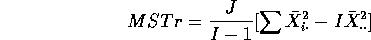
Now examine the Treatment Sum of Squares. First note that
 . Use this to see that the Treatment Sum of Squares
is given by
. Use this to see that the Treatment Sum of Squares
is given by
which simplifies to

This last is the numerator of  .
.