Reading:
See Lecture 18 for plots of the data and Lecture 19 for our first analysis.
We have found that STAY, CULTURE and CHEST are significant and that we must retain one of the three variables BED, NURSES and CENSUS which measure size of the hospital. These three variables are multicollinear. Picking the variable of the three which produces the largest multiple R2 we go with NURSES. Now we look at the question of adding further variables to that 4 covariate model.
> anova(fit.n,fit.full)
Analysis of Variance Table
Response: Risk
 Model   Resid. Df    RSS   Test Df SumSq   F Value    Pr(F)
 FULL       108    95.63982
 REDUCED    104    95.63982    4    2.9895 0.8127053 0.5198417
This suggests we need not consider adding further variables.
However, we should examine diagnostics and consider the question of how variables are likely to influence RISK.
Suggestion: Transform other variables.
Define NURSE.RATIO = NURSES/CENSUS. Idea: large values indicate more intensive nursing care.
Define CROWDING = CENSUS/BEDS. Idea: large values indicate a crowded hospital.
Add these variables to the model.
> Nurse.Ratio <- scenic$Nurse/scenic$Census
> sc.ext <- data.frame(scenic, Nurse.Ratio)
> Crowding <- scenic$Census/scenic$Beds
> sc.ext <- data.frame(sc.ext, Crowding)
> fit.l20 <- lm(Risk ~ Stay + Culture + Chest +
    Nurses + Crowding + Nurse.Ratio, data = sc.ext)
> summary(fit.l20)
Residuals:
    Min      1Q  Median     3Q   Max
 -2.036 -0.6102 0.01268 0.3956 2.798
Coefficients:
              Value Std. Error t value Pr(>|t|)
(Intercept) -1.2762  0.8753    -1.4581  0.1478
       Stay  0.2196  0.0594     3.6983  0.0003
    Culture  0.0424  0.0099     4.2740  0.0000
      Chest  0.0093  0.0055     1.7040  0.0913
     Nurses  0.0014  0.0007     1.9627  0.0523
   Crowding  1.4296  0.9455     1.5121  0.1335
Nurse.Ratio  0.8238  0.3298     2.4979  0.0140

Residual standard error: 0.9359 on 106 df
Multiple R-Squared: 0.5389
F-statistic: 20.65 on 6 and 106 df,
the p-value is 6.661e-16

Correlation of Coefficients:
            (Intercept)    Stay Culture   Chest  Nurses Crowding
       Stay -0.3314
    Culture  0.1738     -0.1725
      Chest -0.1170     -0.3422 -0.3010
     Nurses  0.3162     -0.2737 -0.0803  0.1608
   Crowding -0.7108     -0.2136 -0.0321 -0.0605 -0.3032
Nurse.Ratio -0.6321      0.2561 -0.1365 -0.2548 -0.3056  0.3849
Conclusion: NURSE.RATIO is a useful predictor.
Can we discard CHEST, CROWDING? NURSES marginal but seems reasonable to keep this variable since we are keeping NURSE.RATIO.
fit.l20.t <- lm(Risk ~ Stay + Culture + Nurse.Ratio
      + Nurses, data = sc.ext)
> summary(fit.l20.t)
Residuals:
    Min      1Q  Median     3Q   Max
 -2.214 -0.6387 0.06483 0.5021 2.655

Coefficients:
              Value Std. Error t value Pr(>|t|)
(Intercept) -0.0831  0.6092    -0.1365  0.8917
       Stay  0.2767  0.0549     5.0417  0.0000
    Culture  0.0482  0.0096     5.0311  0.0000
Nurse.Ratio  0.7695  0.2994     2.5701  0.0115
     Nurses  0.0016  0.0007     2.2607  0.0258

Residual standard error: 0.9511 on 108 df
Multiple R-Squared: 0.5149
F-statistic: 28.66 on 4 and 108 df,
         the p-value is 3.331e-16

Correlation of Coefficients:
            (Intercept)    Stay Culture Nurse.Ratio
       Stay -0.8669
    Culture  0.1569     -0.3317
Nurse.Ratio -0.6468      0.3148 -0.2287
     Nurses  0.1916     -0.3356 -0.0521 -0.1851
> anova(fit.l20,fit.l20.t)
Analysis of Variance Table    Response: Risk
Model   Res df   ESS   test df   SS    F  P value
FULL      106   92.852
REDUCED   108   97.689   2      4.84 2.76 0.068
Conclusion: Can discard CHEST, CROWDING but not NURSES.
Remaining Issues
To demonstrate that changing X causes changes in Y we hold all other important variables constant and try experimental units at various settings of X. Variables we don't know about or can't control are equalized between the different levels of X by randomly assigning units to the different values of X.
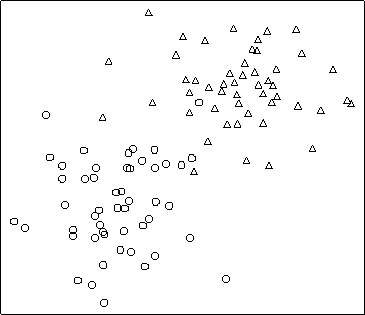
An observational study is one where X cannot be controlled and other variables cannot be held constant. Think about a case where men have generally higher values of both X and Y and women have generally lower values but that among men there is no relation between X and Y Here is a possible plot, the triangles being men.

If you didn't know about the influence of sex you would see a positive correlation between X and Y but if you compute separate correlations for the two groups you see the variables are unrelated. Remember, if you manipulate X in the picture you are either doing so for a women (and X and Y are unrelated for women) or for a man (and again X and Y are unrelated); in either case Y will be unaffected because you would not be affecting the sex of a person.
Doing multiple regression is very much like this. Imagine you have a response variable Y, a variable X whose influence on Y is of primary interest and some other variables which probably influence Y and may influence X as well. You would like to look at the relation between X and Y in groups of cases where all the other covariate values are the same; this is not generally possible. Instead, we estimate the average value of Y for each possible combination of the variable X and the other variables. We ask if this mean depends on X. We say we are adjusting for the other covariates.
The method works pretty well if we have identified all the possible confounding variables so that we can adjust for them all. So, e.g., in our example lowering the nursing ratio would be asserted to lower the risk of nosocomial infection. The trouble is that no such deduction is rigorously possible. You would need to be sure there was not a 3rd variable correlated with both X and Y which is the real cause of variation in both and for which you haven't adjusted. In randomized designed experiments this possibility is dealt with by the randomization.
The slope in a regression model corresponding to X measures the change expected in Y when X is changed by 1 unit and all the other variables in the regression are held constant. It is in this sense the regression method is used to adjust for the other covariates. Researchers say things like "Adjusted for Length of service and publication rate sex has no impact on salary of professors."