Postscript version of these questions

STAT 350

Assignment 3: Solutions

The data and assignment comments are here

1.

Vehicle mileage vs emissions.

(a)

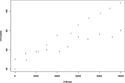
Plot the data.

(b)

Consider the following 4 models for the data:

i.

Two straight lines, one for each vehicle, with different slopes and intercepts,

ii.

Two parallel straight lines.

iii.

Two lines with the same intercept but different slopes.

iv.

One straight line.

Write out model equations for data points number 2 and 22 for the first 3 models.

FIRST MODEL

$$Y_2 = \beta_1 + 1000\beta_2 +\epsilon_2$$

and

$$Y_{22} = \beta_3 + 10000\beta_4 +\epsilon_{22} \, .$$

Here $\beta_1$ and $\beta_3$ are the two intercepts while $\beta_2$ and $\beta_4$ are the slopes.

SECOND MODEL

$$Y_2 = \beta_1 + 1000\beta_2 +\epsilon_2$$

and

$$Y_{22} = \beta_3 + 10000\beta_2 +\epsilon_{22} \, .$$

Here $\beta_1$ and $\beta_3$ are the two intercepts while $\beta_2$ is the common slope.

THIRD MODEL

$$Y_2 = \beta_1 + 1000\beta_2 +\epsilon_2$$

and

$$Y_{22} = \beta_1 + 10000\beta_4 +\epsilon_{22} \, .$$

Here $\beta_2$ and $\beta_4$ are the two slopes while $\beta_1$ is the common intercept.

(c)

Fit all 4 models. Hand in: estimates of the slopes and intercepts and of $\sigma$. Do NOT just hand in output from SAS or Minitab.

I create a data file which contains the design matrix for the first model.

  50 1     0        0     0 
  56 1  1000        0     0 
  58 1  2000        0     0
  60 1  3000        0     0
  58 1  4200        0     0
  63 1  5000        0     0
  73 1  6000        0     0
  71 1  6900        0     0
  76 1  8000        0     0
  73 1  9200        0     0
  80 1 10000        0     0
  40 0     0        1     0 
  49 0     0        1  1100  
  58 0     0        1  2200 
  65 0     0        1  3000 
  75 0     0        1  4000
  77 0     0        1  5300
  86 0     0        1  6000
  93 0     0        1  7000
  98 0     0        1  8100
 103 0     0        1  9000
 109 0     0        1 10000

I used the following SAS code to fit the models.

options pagesize=60 linesize=80;
data mileage;
  infile 'mile1.dat' ;
  input emiss car1 mile1 car2 mile2 ;
  mile = mile1+mile2;
proc glm  data=mileage;
   model emiss =  car1 mile1 car2 mile2 / NOINT ;
   estimate 'sloped' mile1 1 mile2 -1 /E ;
   estimate 'intd' car1 1 car2 -1 /E ;
run ;
proc glm  data=mileage; 
   model emiss =  car1 car2 mile /NOINT  ; 
run ;
proc glm  data=mileage; 
   model emiss =  mile1 mile2  ; 
run ;
proc glm  data=mileage; 
   model emiss =  mile ; 
run ;
proc glm  data=mileage;
   model emiss =  car1 mile1 car2 mile2 / NOINT ;
   estimate 'veh1em' car1 10000 mile1 50000000 /E ;
   estimate 'veh2em' car2 10000 mile2 50000000 /E ;
   estimate 'diff'   car1 10000 mile1 50000000 
         car2 -10000 mile2 -50000000 /E;
run ;

Here are the estimates;

Model	$\hat\beta_1$	$\hat\beta_2$	$\hat\beta_3$	$\hat\beta_4$	$\hat\sigma$
1	51.28	0.00278	42.93	0.00684	2.79
2	41.20	0.00479	53.29	--	7.41
3	47.16	0.00337	--	0.00623	3.62
4	47.19	0.00480	--	--	9.61

(d)

Using formal hypothesis tests and plots select the best of these models. Again, I do not want computer output but discussion. You may attach computer output in order to say things like: ``The Sum of Squares for ... is on page ..." and to hand in plots on which you comment in the discussion but I will not be looking through the output.

I begin by testing the hypothesis that $\beta_2 = \beta_4$. You can do this either using the extra sum of squares F-test or a suitable t-test. The line estimate 'sloped' gets standard errors and a t-statistic. The output lines corresponding to the estimate lines is

                      T for H0: Pr > |T| Std Error of
Parameter  Estimate Parameter=0              Estimate

sloped  -0.00405367    -10.75     0.0001   0.00037706
intd     8.35473800      3.72     0.0016   2.24468995

Each of these tests is quite significant so that you can't get by with either a common slope or a common intercept. That is, the first model is preferred. You can also do extra sum of squares tests. The needed information is in the Error SS from the various runs of glm:

MODEL     Error DF     Error SS          MSE
1           18        140.47791         7.80433
2           19       1042.46491        54.86657
3           19        248.59354        13.0838705
4           20       1847.50378        92.3751888

The extra SS F-statistic for testing model 2 against model 1 is [(1042.46-140.48)/1]/[140.48/18] and this is compared to F tables with 1 and 18 degrees of freedom. The statistic value is 115.6 which is very significant. Similarly model 3 is rejected in favour of model 1. Model 4, requiring both models 2 and 3 to be correct is untenable. It can be tested directly against model 1 using [(1847.50378-140.477910/2]/7.80433 as an F-test.

(e)

For the final selected model estimate the total emissions of CO in grams for each vehicle over the first 10000 miles. (This is the area under the fitted straight line from 0 to 10000 and is a linear combination of the parameter estimates.) Attach a standard error.

In terms of the coefficients in the model the emissions for vehicle1 are $10,000\beta_1 + 50,000,000\beta_2$ while those for vehicle 2 are $10,000\beta_3 + 50,000,000\beta_4$. These are estimated by plugging in least squares estimates. These two estimates and their difference are all linear combinations of the form $a^T\hat\beta$ for which the standard error is $\sigma\sqrt{a^t(X^TX)^{-1} a}$. You can calculate these standard errors using estimate statements as in the last run of proc glm. The corresponding output is

                      T for H0:  Pr > |T| Std Error of
Parameter   Estimate Parameter=0             Estimate

veh1em    651968.435      77.40   0.0001    8423.4004
veh2em    771104.319      91.53   0.0001    8424.8153
diff     -119135.884     -10.00   0.0001   11913.4876

The last line shows that the two cars have different emissions in total over the first 10000 miles (answering the next part) while the previous 2 permit confidence intervals of the form $651968\pm t_{18,0.025} 8423$.

(f)

Are the emissions of the two vehicles different over the first 10000 miles?

The answer is yes, the second vehicle clearly has higher emissions. See the previous question for the test.

(g)

Suppose the two cars are of the same make but that one vehicle was equipped with a special pollution control device. In 4 or 5 sentences comment on the experimental design as a method of determining whether or not the device reduces emissions and on what else you would want to find out from the experimenter to help interpret the results.

The key problem is replication. In any case we need to be sure that the two cars are similar in make, model, driver, road conditions, nature and extent of maintenance and so on. The trouble is that with only two cars the variation from car to car under identical conditions cannot be allowed for. How do you know that if you took 2 cars identically equipped with no different pollution control devices you wouldn't see just as big a difference?

2.

Data below are from a nitrogen balance experiment on Kangaroo Island Wallabies, taken from Barker,S. (1968). ``Nitrogen balance and Water Intake in the Kangaroo Island Wallaby'' Austral. J. Experimental Biology and Medical Science, 46, 17-32.

Y	X1	X2	X3	X4
Nitrogen	Body	Dry	Water	Nitrogen
Excreted	Weight	Intake	Intake	Intake
162	3.386	16.6	41.7	54
174	3.033	18.1	40.9	99
119	3.477	13.4	25.0	46
205	3.278	22.6	39.2	188
312	3.368	26.5	47.4	345
157	2.932	21.4	51.6	66
184	3.128	30.3	71.6	171
155	3.251	17.6	27.1	81
192	3.396	21.3	37.7	175
331	3.497	29.9	50.5	399
114	3.182	12.8	28.4	38
159	3.234	19.6	34.3	106
260	3.139	36.2	77.6	228
265	3.434	35.0	58.9	291
387	2.970	32.9	55.3	449
146	3.230	22.9	46.2	72
233	3.470	32.9	67.4	176
261	3.000	35.7	77.1	235
287	3.224	34.4	74.9	288
412	3.366	36.2	60.7	485
174	3.264	29.9	65.4	92
171	3.292	21.7	51.2	126
259	3.525	35.0	66.8	224
298	3.036	29.7	65.8	276
407	3.356	29.2	48.1	386

Fit the model

$$E(Y) = \beta_0 + \beta_1 X_1 + \beta_2 X_2 + \beta_3 X_3 + \beta_4 X_4$$

by least squares. Get estimates and standard errors for all the parameters and an estimate of $\sigma$. Suggest a simpler model for the data, and fit it. Check the fit of the model, graphically and, if the model seems poor, modify it appropriately. Hand in a discussion of your findings bolstered by output used only as an appendix. I will be marking the discussion, not sorting through the output.

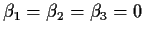
The final fitted model has X₄ only. An extra sum of squares F-test comparing this test to the full model accepts the null hypothesis that $\beta_1=\beta_2=\beta_3=0$. The plots look quite alright though observation 25 has a surprisingly large residual. Deletion of this observation changes the conclusions, however; variable X₃ is retained.

Here is SAS code and output.