![\begin{displaymath}\left[
\begin{array}{rr}
1 & -2 \\
1 & -1 \\
1 & 0 \\
1 & 1 \\
1 & 2
\end{array}\right] \, .
\end{displaymath}](img1.gif)
If we fit a simple linear regression of the form
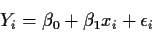
for which the design matrix is as above, evaluate the non-centrality parameter of the t test of
 when in fact
  and
and
 .
What would the power of a
two sided 1% level t test of this null hypothesis be? How many
times would we have to replicate this design to get a power of 0.9 for
a 1% level test?
.
What would the power of a
two sided 1% level t test of this null hypothesis be? How many
times would we have to replicate this design to get a power of 0.9 for
a 1% level test?
Solution:
We have
![\begin{displaymath}X^TX = \left[
\begin{array}{rr}
5 & 0 \\
0 & 10
\end{array}\right]
\end{displaymath}](img6.gif)
and
![\begin{displaymath}(X^TX)^{-1} =\left[
\begin{array}{rr}
\frac{1}{5} & 0 \\
0 & \frac{1}{10}
\end{array}\right] \, .
\end{displaymath}](img7.gif)
The variance of
 is
is
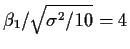
 and the non-centrality
parameter is
and the non-centrality
parameter is
 .
From Table B 5 p 1347 I get
a power of 0.31 (3 df for error). If we replicate the design m times we
would have a non-centrality parameter of
.
From Table B 5 p 1347 I get
a power of 0.31 (3 df for error). If we replicate the design m times we
would have a non-centrality parameter of  .
The infinity line in
the table would suggest an m of 1 but because the degrees of freedom is
so low we have to do some trial and error. An m of 2 would give a
non-centrality parameter of 5.66. There would be 8 degrees of freedom and
the power would be around 0.95 so m=2 would be adequate.
.
The infinity line in
the table would suggest an m of 1 but because the degrees of freedom is
so low we have to do some trial and error. An m of 2 would give a
non-centrality parameter of 5.66. There would be 8 degrees of freedom and
the power would be around 0.95 so m=2 would be adequate.
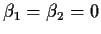 in the model

Assume that in fact
 and
and
 .
.
Solution: The non-centrality parameter is
![\begin{displaymath}E(RegressionSS)/\sigma^2 - 2 =
[\beta_1, \beta_2] X_2^T (I-H_1)X_2 [\beta_1,\beta_2]^T/\sigma^2
\end{displaymath}](img16.gif)
Here X1=[1,1,1,1,1]T, H1 = X1 (X1TX1)X1T is a
 matrix with all entries
equal to 1/5
and
matrix with all entries
equal to 1/5
and
![\begin{displaymath}X_2 =\left[
\begin{array}{rr}
-2 & 2\\
-1 &-1 \\
0 & -2\\
1 &-1 \\
2 & 2
\end{array}\right] \, .
\end{displaymath}](img18.gif)
We find
![$[\beta_1,\beta_2]X_2^T = [2,-3,-4,-1,6]$](img19.gif) and finally
that the non-centrality parameter is 66/2.5=26.4.
and finally
that the non-centrality parameter is 66/2.5=26.4.
The data set in the text has one number different than the data set on the computer disk. The results below are for the data off the disk. Students who took the data from the book got somewhat different results but I marked them right, since they were right for the data they used.
Solution:
The fitted line is

a) The residual plot is
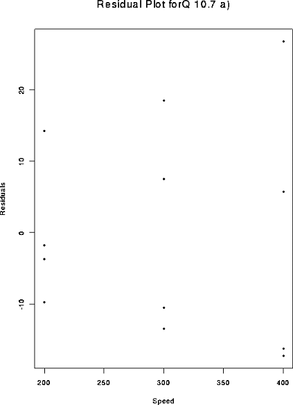
This plot suggests that the residuals are bigger when Speed is bigger; this is evidence of heteroscedasticity.
c) The desired plot is
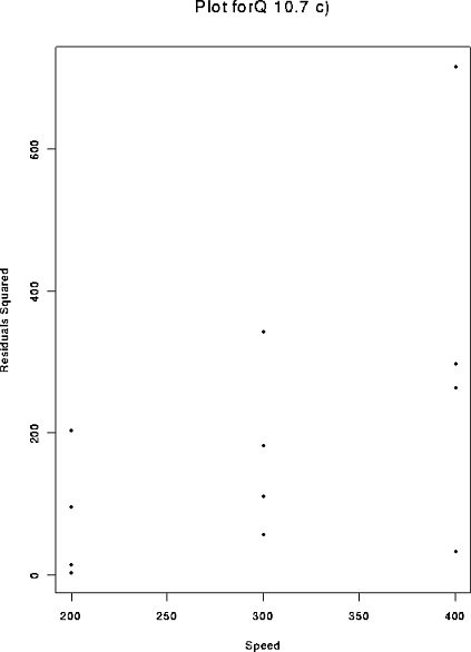
This plot suggests a linear fit of
 against Speed might
work.
against Speed might
work.
d) The regression equation is

The required weights are
 0.0146 0.0032 0.0052 0.0032 0.0146 0.0052
 0.0052 0.0032 0.0146 0.0032 0.0146 0.0052
e) The weighted least squares regression line is

These estimates are little changed compared to the standard errors.
| OLS | WLS | OLS | WLS | |
| Parameter | Estimate | Estimate | SE | SE |
| Intercept | -5.75 | -6.23 | 16.73 | 13.17 |
| Slope | 0.1875 | 0.1891 | 0.0538 | 0.0506 |
f) The standard errors from weighted least squares are rather smaller though more so for the less important parameter, the intercept.

where the errors
 have variances
 and
the wi are known quantities.
Find an explicit algebraic formula for the weighted least squares
estimate of
and
the wi are known quantities.
Find an explicit algebraic formula for the weighted least squares
estimate of  .
.
Solution: The matrix X is a single column of n ones.
The matrix W is diagonal with wi down the diagonal. The vector
WX has entries
 and finally
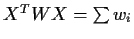 .
Next XTWY is the inner product between the vector
WX with ith entry wi and Y with ith entry Yi so
.
Next XTWY is the inner product between the vector
WX with ith entry wi and Y with ith entry Yi so
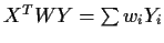 .
Finally
.
Finally
 which is what is
called a weighted average.
which is what is
called a weighted average.