Postscript version of these notes
STAT 801 Lecture 25
Reading for Today's Lecture:
Goals of Today's Lecture:
- Do Bayesian estimation examples.
- Look at hypothesis testing as decision theory.
Bayesian estimation
Now let's focus on the problem of estimation of a 1 dimensional
parameter. Mean Squared Error
corresponds to using
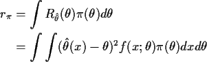
The risk function of a procedure (estimator)
 is
is
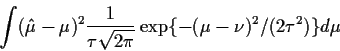
Now consider using a prior with density
 .
The
Bayes risk of
is
.
The
Bayes risk of
is
How should we choose
to minimize  ? The solution
lies in recognizing that
? The solution
lies in recognizing that
 is really a joint
density
is really a joint
density
For this joint density the conditional density of X given  is just the model
 .
From now on I write the model as
.
From now on I write the model as
 to emphasize this fact. We can now compute
a different way by factoring the joint density a different way:
to emphasize this fact. We can now compute
a different way by factoring the joint density a different way:
where now f(x) is the marginal density of x and
 denotes the conditional density of
given X. We call
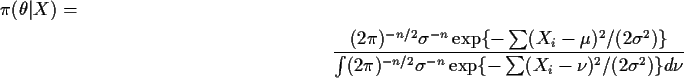
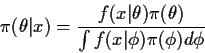
the posterior density. It is found via
Bayes theorem (which is why this is Bayesian statistics):
denotes the conditional density of
given X. We call
the posterior density. It is found via
Bayes theorem (which is why this is Bayesian statistics):
With this notation we can write
Now we can choose
 separately for each x to minimize the
quantity in square brackets (as in the NP lemma). The quantity in
square brackets is a quadratic function of
and can be seen
to be minimized by
separately for each x to minimize the
quantity in square brackets (as in the NP lemma). The quantity in
square brackets is a quadratic function of
and can be seen
to be minimized by
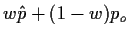
which is
and is called the posterior expected mean of .
Example: Consider first the problem of estimating a normal
mean  .
Imagine, for example that
is the true speed of sound.
I think this is around 330 metres per second and am pretty sure that I
am within 30 metres per second of the truth with that guess. I might
summarize my opinion by saying that I think
has a normal distribution
with mean
.
Imagine, for example that
is the true speed of sound.
I think this is around 330 metres per second and am pretty sure that I
am within 30 metres per second of the truth with that guess. I might
summarize my opinion by saying that I think
has a normal distribution
with mean  330 and standard deviation
  .
That is, I take a
prior density
.
That is, I take a
prior density  for
to be
for
to be
 .
Before I make any
measurements my best guess of
minimizes
.
Before I make any
measurements my best guess of
minimizes
This quantity is minimized by the prior mean of ,
namely,
Now suppose we collect 25 measurements of the speed of sound. I will
assume that the relationship between the measurements and
is that
the measurements are unbiased and that the standard deviation of the
measurement errors is  which I assume that we know. Thus the
model is that conditional on
which I assume that we know. Thus the
model is that conditional on
 are iid
 .
The joint density of the data and
is then
.
The joint density of the data and
is then
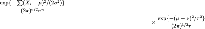
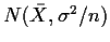
Thus
 .
Conditional distribution of
given
is
normal.
.
Conditional distribution of
given
is
normal.
Use standard MVN formulas to calculate
conditional means and variances.
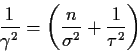
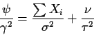
Alternatively the exponent in the
joint density is of the form
plus terms not involving
where
and
This means that the conditional density of
given the data is
 .
In other words the posterior mean of
is
.
In other words the posterior mean of
is
which is a weighted average of the prior mean  and the sample
mean
and the sample
mean  .
Notice that the weight on the data is large when n
is large or
.
Notice that the weight on the data is large when n
is large or  is small (precise measurements) and small when
 is small (precise prior opinion).
Improper priors: When the density does not integrate
to 1 we can still follow the machinery of Bayes' formula to derive
a posterior. For instance in the
example consider
the prior density
 .
This ``density'' integrates
to
.
This ``density'' integrates
to  but using Bayes' theorem to compute the posterior would
give
but using Bayes' theorem to compute the posterior would
give
It is easy to see that this cancels to the limit of the case previously
done when
 giving a
 density.
That is, the Bayes estimate of
for this improper prior is .
density.
That is, the Bayes estimate of
for this improper prior is .
Admissibility: Bayes procedures corresponding to proper priors are
admissible. It follows that for each
 and each real
the estimate
and each real
the estimate
is admissible. That this is also true for w=1, that is, that is admissible is much harder to prove.
Minimax estimation: The risk function of is simply
 .
That is, the risk function is constant since
it does not depend on .
Were
Bayes for a proper
prior this would prove that
is minimax. In fact this is also
true but hard to prove.
.
That is, the risk function is constant since
it does not depend on .
Were
Bayes for a proper
prior this would prove that
is minimax. In fact this is also
true but hard to prove.
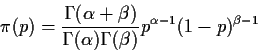
Example: Given p X has a Binomial(n,p)
distribution. Give p a Beta
 prior density
The joint ``density'' of X and p is
posterior density of p given X is of the form
for a suitable normalizing constant c. This is
Beta
 density.
Mean of Beta
distribution is
density.
Mean of Beta
distribution is
 .
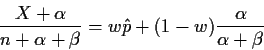
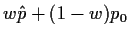
So Bayes estimate
of p is
.
So Bayes estimate
of p is
where
 is usual mle.
Notice: weighted average of prior mean and
mle. Notice prior is proper for
is usual mle.
Notice: weighted average of prior mean and
mle. Notice prior is proper for  and
and
 .
To get w=1 take
.
To get w=1 take
 and use improper
prior
and use improper
prior
Again we learn that each
 is admissible for
.
Again
is admissible for
.
Again  is admissible but
our theorem is not adequate to prove this fact.
is admissible but
our theorem is not adequate to prove this fact.
The risk function of
 is
is
which is
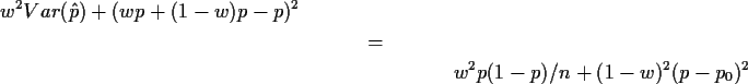
Risk function constant if coefficients of
p2 and p in risk are 0. Coefficient of
p2 is
-w2/n +(1-w)2
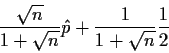
so
w=n1/2/(1+n1/2). Coefficient of p is then
w2/n -2p0(1-w)2
which vanishes if 2p0=1 or p0=1/2. Working
backwards we find that to get these values for w and p0
we require
 .
Moreover
.
Moreover
w2/(1-w)2 = n
gives
or
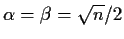 .
Minimax estimate of
p is
.
Minimax estimate of
p is
Example: Now suppose that
are iid
 with
with  known. Consider as the improper prior for
which is constant. The
posterior density of
given X is then
known. Consider as the improper prior for
which is constant. The
posterior density of
given X is then
 .
.
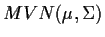
For multivariate estimation it is common to extend the notion of squared error loss
by defining
For this loss function the risk is the sum of the MSEs
of the individual components and
the Bayes estimate is the posterior mean again.
Thus
is Bayes for an improper
prior in this problem.
It turns out that
is minimax; its risk function is
the constant
 .
If the dimension p of
is 1 or 2 then
is also admissible but if
.
If the dimension p of
is 1 or 2 then
is also admissible but if  then it is inadmissible.
This fact was first demonstrated by James and Stein who
produced an estimate which is better,
in terms of this risk function, for every .
The ``improved'' estimator, called the
James Stein estimator is essentially never used.
then it is inadmissible.
This fact was first demonstrated by James and Stein who
produced an estimate which is better,
in terms of this risk function, for every .
The ``improved'' estimator, called the
James Stein estimator is essentially never used.
Hypothesis Testing and Decision Theory
Decision analysis of hypothesis testing takes
 and
and
or more generally
 and
and
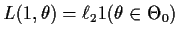 for two positive
constants
for two positive
constants  and
and  .
We make the decision space convex
by allowing a decision to be a probability measure on D. Any such measure
can be specified by
.
We make the decision space convex
by allowing a decision to be a probability measure on D. Any such measure
can be specified by
 so
so
![${\cal D} =[0,1]$](img83.gif) .
The
loss function of
.
The
loss function of
![$\delta\in[0,1]$](img84.gif) is
is
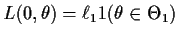
Simple hypotheses: Prior is  and
and  with
with
 .
.
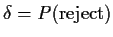
Procedure: map from sample space to  - a test function.
Risk function of procedure  is a pair of numbers:
and
We find
and
The Bayes risk of  is
is
We saw in the hypothesis testing section that this is minimized
by
which is a likelihood ratio test. These tests are Bayes
and admissible. The risk is constant if
 ;
you can use this to find the minimax test in this context.
;
you can use this to find the minimax test in this context.
Richard Lockhart
2000-03-21
![\begin{displaymath}r_\pi(\hat\theta) = \int \left[ \int (\hat\theta(x) - \theta)^2
\pi(\theta\vert x) d\theta \right] f(x) dx
\end{displaymath}](img16.gif)