Postscript version of these notes

STAT 804: Notes on Lecture 3

Definition: If $\{\epsilon_t\}$ is a white noise series and $\mu$ and $b_0,\ldots,b_p$ are constants then

$$X_t = \mu + b_0\epsilon_t + b_1 \epsilon_{t-1} + \cdots + b_p \epsilon_{t-p}$$

is a moving average of order p; we write MA(p).

Question: From observations on X can we estimate the b's and $\sigma^2=\text{Var}(\epsilon_t)$ accurately? NO.

Definition: A model for data X is a family $\{P_\theta; \theta\in\Theta\}$ of possible distributions for X.

Definition: A model is identifiable if $\theta_1 \neq \theta_2$ implies that $P_{\theta_1} \neq P_{\theta_2}$; that is different $\theta$'s give different distributions for the data.

When a model is unidentifiable there are different values of $\theta$which make exactly the same predictions about the data so the data do not permit you to distinguish between these $\theta$ values.

Example: Suppose $\epsilon$ is an iid $N(0,\sigma^2)$ series and that $X_t = b_0 \epsilon_t + b_1 \epsilon_{t-1}$. Then the series X has mean 0 and covariance

$$C_X(h) = \begin{cases} (b_0^2+b_1^2) \sigma^2 & h=0 \\ b_0 b_1 \sigma^2 & h=1 \\ 0 & \text{otherwise} \end{cases}$$

Now a normal distribution is specified by its mean and its variance so two normal time series with mean 0 and the same covariance function have the same distribution. You can see that if you multiply the $\epsilon$'s by a and divide both b₀ and b₁ by a then the covariance function of X is unchanged. Thus we cannot hope to estimate all three parameters, b₀, b₁ and $\sigma$. We choose to set the parameter b₀ to be 1. Now are the parameters b₁ and $\sigma$identifiable? We try to solve the equations

$$C(0) = (1+b^2) \sigma^2$$

and

$$C(1) = b\sigma^2$$

to see if the solution is unique. Divide the two equations to see

$$\frac{C(1)}{C(0)} = \frac{b}{1+b^2}$$

or

$$b^2 - \frac{C(0)}{C(1)} b + 1 = 0$$

which has the solutions

$$\frac{ \frac{C(0)}{C(1)} \pm \sqrt{\left( \frac{C(0)}{C(1)}\right)^2 - 4}}{ 2}$$

You should notice two things:

1.

If

$$\left\vert \frac{C(0)}{C(1)}\right\vert > 2$$

there are no solutions. Since $C(0) = \sqrt{\text{Var}(X_t) \text{Var}(X_{t+1})}$ we can see that C(1)/C(1) is the correlation between X_t and X_t+1. We have proved that for an MA(1) process this correlation cannot be more than 1/2 in absolute value.

2.

If

$$\left\vert \frac{C(0)}{C(1)}\right\vert < 2$$

there are two solutions.

The two solutions multiply together to give the constant term 1 in the quadratic equation. If the two roots are distinct it follows that one of them is larger than 1 and the other smaller in absolute value. Let b and b^* denote the two roots. Let $\alpha = C(1)/b$ and $\alpha^* =C(1)/b^*$. Let $\epsilon_t$ be iid $N(0,\alpha)$ and $\epsilon_t^*$ be iid $N(0,\alpha^*)$. Then

$$X_t \equiv \epsilon_t + b \epsilon_{t-1}$$

and

$$X_t^* \equiv \epsilon_t + b^* \epsilon_{t-1}^*$$

have identical means and covariance functions. Observing X_t you cannot distinguish the first of these models from the second. We will fit MA(1) models by requiring our estimated b to have $\vert\hat{b}\vert \le 1$.

Reason: We can manipulate the model equation for Xjust as we did for and autoregressive process last time:
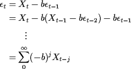
$$\begin{align*}\epsilon_t & = X_t - b \epsilon_{t-1} \\ & = X_t - b(X_{t-1}-b\ep... ...ilon_{t-1} \\ & \qquad \vdots \\ & = \sum_0^\infty (-b)^j X_{t-j} \end{align*}$$
This manipulation makes sense if |b| < 1. If so then we can rearrange the equation to get

$$X_t =\epsilon_t - \sum_1^\infty (-b)^j X_{t-j}$$

which is an autoregressive process.

If, on the other hand, |b| > 1 then we can write

$$X_t = b(\frac{1}{b} \epsilon_t -\epsilon_{t-1})$$

Let $\epsilon_t^* = \epsilon_t/b$; $\epsilon^*$ is also white noise. We find
$$\begin{align*}\epsilon_{t-1}^* & = X_t - \frac{1}{b} \epsilon_{t}^* \\ & = X_t ... ... \\ & \qquad \vdots \\ & = \sum_0^\infty (-\frac{1}{b})^j X_{t+j} \end{align*}$$
which means

$$X_t = \epsilon_{t-1}^* - \sum_1^\infty (-\frac{1}{b})^j X_{t+j}$$

This represents the current value as depending on the future which seems physically far less natural than the other choice.

Definition: An MA(p) process is invertible if it can be written in the form

$$X_t = \sum_1^\infty a_j X_{t-j}+\epsilon_t$$

Definition: A process X is an autoregression of order p (written AR(p)) if

$$X_t = \sum_1^p a_j X_{t-j}+\epsilon_t$$

(so an invertible MA is an infinite order autoregression).

Definition: The backshift operator transforms a time series into another time series by shifting it back one time unit; if X is a time series then BX is the time series with

$$(BX)_t = X_{t-1}\, .$$

The identity operator I satisfies IX=X. We use B^j for $j=1,2,\ldots$to denote B composed with itself j times so that

(B^jX)_t = X_t-j

For j=0 this gives B⁰=I.

Now we use B to develop a formal method for studying the existence of a given AR(p) and the invertibility of a given MA(p). An AR(1) process satisfies

$$(I-a_1B)X = \epsilon$$

If you think of I-a₁B as some sort of infinite dimensional matrix then you get the formal identity

$$X = (I-a_1B)^{-1}\epsilon$$

So how will we define this inverse of an infinite matrix? We use the idea of a geometric series expansion.

If b is a real number then

$$(1-ab)^{-1} =\frac{1}{1-ab} = \sum_{j=0}^\infty (ab)^j$$

so we hope that (I-a₁B)^-1 can be defined by

$$(I-a_1B)^{-1} = \sum_{j=0}^\infty a_1^j B^j$$

This would mean

$$X = \sum_{j=0}^\infty a_1^j B^j \epsilon$$

or looking at the formula for a particular tand remembering the meaning of B^j we get

$$X_t = \sum_{j=0}^\infty a_1^j \epsilon_{t-j}$$

This is the formula I had in lecture 2.

Now consider a general AR(p) process:

$$(I-\sum_1^p a_j B^j)X = \epsilon$$

We will factor the operator applied to x. Let

$$\phi(x) = 1- \sum_1^p a_j x^j$$

Then $\phi$ is a polynomial of degree p. It thus has (a theorem of C. F. Gauss) p roots $1/b_1,\ldots,1/b_p$. (None of the roots is 0 because the constant term in $\phi$ is 1.) This means we can factor $\phi$ as

$$\phi(x) = \prod_1^p (1-b_j x)$$

Now back to the definition of X:

$$\prod_1^p(I-b_jB) X = \epsilon$$

can be solved by inverting each term in the product (in any order -- the terms in the product commute) to get

$$X = \prod_1^p(I-b_jB)^{-1}\epsilon$$

The inverse of I-b₁B will exist if the sum

$$\sum_{k=0}^\infty b_j^k B^k$$

converges; this requires |b_j| < 1. Thus a stationary AR(p) solution of the equations exists if every root of the characteristic polynomial $\phi$ is larger than 1 in absolute value (actually the roots can be complex and I mean larger than 1 in modulus).

Summary

• An MA(q) process $X_t = \epsilon_t - \sum_{j=1}^q b_j \epsilon_{t-j}$is invertible if and only if all roots of the characteristic polynomial $\psi(x) = 1 - \sum_{j=1}^q b_j x^j$ lie outside the unit circle in the complex plain.

• For a given covariance function of an MA(q) process there is only one set of coefficients $b_1,\ldots,b_q$ for which the process is invertible.

• An AR(p) process $X_t - \sum_{j=1}^q a_j X_{t-j} = \epsilon_t$ is asymptotically stationary if and only if all roots of the characteristic polynomial $\phi(x) = 1-\sum_1^p a_j x^j$ lie outside the unit circle in the complex plain.

  (Asymptotically stationary means this: if you make $X_{-1},X_{-2}, \ldots,X_{-p}$ anything at all and use the equation defining the AR(p)to define all the rest of the X values then as $t\to\infty$ the process gets closer to being stationary. The assertion of asymptotic stationarity is equivalent here to the existence of an exactly stationary solution of the equations.)

Definition: A process X is an ARMA(p,q) (mixed autoregressive of order pand moving average of order q) if it satisfies

$$\phi(B) X = \psi(B)\epsilon$$

where $\epsilon$ is white noise and

$$\phi(B) = I - \sum_1^p a_j B^j$$

and

$$\psi(B) = I - \sum_1^p b_j B^j$$

The ideas we used above can be stretched to show that the process X is identifiable and causal (can be written as an infinite order autoregression on the past) if the roots of $\psi(x)$ lie outside the unit circle. A stationary solution, which can be written as an infinite order causal (no future $\epsilon$s in the average) moving average, exists if all the roots of $\phi(x)$ lie outside the unit circle.

Other Stationary Processes:

1.

Periodic processes. Suppose Z₁ and Z₂ are independent $N(0,\sigma^2)$ random variables and that $\omega$ is a constant. Then

$$X_t = Z_1 \cos(\omega t) + Z_2 \sin(\omega t)$$

has mean 0 and
$$\begin{align*}\text{Cov}(X_t,X_{t+h}) & = \sigma^2 \left[\cos(\omega t)\cos(\ome... ...n(\omega t)\sin(\omega(t+h))\right] \\ & = \sigma^2 \cos(\omega h) \end{align*}$$
Since X is Gaussian we find that X is second order and strictly stationary. In fact (see your homework) You can write

$$X_t = R \sin(\omega t+\Phi)$$

where R and $\Phi$ are suitable random variables so that the trajectory of X is just a sine wave.

2.

Poisson shot noise processes:

A Poisson process is a process N(A) indexed by subsets A of the real line with the property that each N(A) has a Poisson distribution with parameter $\lambda\text{length}(A)$ and if $A_1,\ldots A_p$ are any non-overlapping subsets of R then $N(A_1),\ldots, N(A_p)$ are independent. We often use N(t) for N([0,t]).

To define a shot noise process we let X(t) =1 at those t where there is a jump in N and 0 elsewhere. The process X is stationary. If we have some function g defined on $[0,\infty)$ and decreasing sufficiently quickly to 0 (like say g(x) =e^-x) then the process

$$Y(t) = \sum g(t-\tau) 1(X(\tau)=1) 1(\tau \le t)$$

is stationary. It has a jump every time t passes a jump in the Poisson process and otherwise follows the trajectory of the sum of several copies of g (shifted around in time). We commonly write

$$Y(t) = \int_0^\infty g(t-\tau) dN(\tau)$$