8. Simple Linear Regression¶

8.1. Preliminaries¶

import pandas as pd
con = pd.read_csv('Data/ConcreteStrength.csv')
con.rename(columns={'Fly ash': 'FlyAsh', 'Coarse Aggr.': "CoarseAgg",
                    'Fine Aggr.': 'FineAgg', 'Air Entrainment': 'AirEntrain', 
                    'Compressive Strength (28-day)(Mpa)': 'Strength'}, inplace=True)
con['AirEntrain'] = con['AirEntrain'].astype('category')
con.head()

	No	Cement	Slag	FlyAsh	Water	SP	CoarseAgg	FineAgg	AirEntrain	Strength
0	1	273.0	82.0	105.0	210.0	9.0	904.0	680.0	No	34.990
1	2	163.0	149.0	191.0	180.0	12.0	843.0	746.0	Yes	32.272
2	3	162.0	148.0	191.0	179.0	16.0	840.0	743.0	Yes	35.450
3	4	162.0	148.0	190.0	179.0	19.0	838.0	741.0	No	42.080
4	5	154.0	112.0	144.0	220.0	10.0	923.0	658.0	No	26.820

8.2. Linear regression with a single explanatory variable¶

There are many ways to do linear regression in Python. We have already used the heavyweight Statsmodels library, so we will continue to use it here. It has much more functionality than we need, but it provides nicely-formatted output similar to SAS Enterprise Guide.

The method we will use to create linear regression models in the Statsmodels library is OLS(). OLS stands for “ordinary least squares”, which means the algorithm finds the best fit line my minimizing the squared residuals (this is “least squares”). The “ordinary” part of the name gives us the sense that the type of linear regression we are seeing here is just the tip of the methodological iceberg. There is a whole world of non-ordinary regression techniques out there intended to address this or that methodological problem or circumstance. But since this is a basic course, we will stick with ordinary least squares.

8.2.1. Preparing the data¶

Recall the general format of the linear regression equation: \(Y = \beta_0 + \beta_1 X_1 + ... + \beta_n X_n\), where \(Y\) is the value of the response variable and \(X_i\) is the value of the explanatory variable(s).

If we think about this equation in matrix terms, we see that Y is a 1-dimensional matrix: it is just a single column (or array or vector) of numbers. In our case, this vector corresponds to the compressive strength of different batches of concrete measured in megapascals. The right-hand side of the equation is actually a 2-dimensional matrix: there is one column for our X variable and another column for the constant. We don’t often think about the constant as a column of data, but the Statsmodels library does, which is why we are talking about it.

Creating a linear regression model in Statsmodels thus requires the following steps:

Import the Statsmodels library
Define Y and X matrices. This is optional, but it keeps the OLS() call easier to read
Add a constant column to the X matrix
Call OLS() to define the model
Call fit() to actually estimate the model parameters using the data set (fit the line)
Display the results

Let’s start with the first three steps:

import statsmodels.api as sm
Y = con['Strength']
X = con['FlyAsh']
X.head()

  105.0
  191.0
  191.0
  190.0
  144.0
Name: FlyAsh, dtype: float64

We see above that X is a single column of numbers (amount of fly ash in each batch of concrete). The numbers on the left are just the Python index (very row in a Python array has a row number, or index).

8.2.2. Adding a column for the constant¶

We can add another column for the regression constant using Statsmodels add_constant() method:

X = sm.add_constant(X)
X.head()

	const	FlyAsh
0	1.0	105.0
1	1.0	191.0
2	1.0	191.0
3	1.0	190.0
4	1.0	144.0

Notice the difference: the X matrix has been augmented with a column of 1s called “const”. To see why, recall the point of linear regression: to use data to “learn” the parameters of the best-fit line and use the parameters to make predictions. The parameters of a line are its y-intercept and slope. Once we have the y-intercept and slope (\(\beta_0\) and \(\beta_1\) in the equation above or b and m in grade 9 math), we can multiply them by the data in the X matrix to get a prediction for Y.

Written out in words for the first row of our data, we get: Concrete strength estimate = \(\beta_0\) x 1 + \(\beta_1\) x 105.0

The “const” column simply provides a placeholder—a bunch of 1s to multiply the constant by. So now we understand why we have to run add_constant().

8.2.3. Running the model¶

model = sm.OLS(Y, X, missing='drop')
model_result = model.fit()
model_result.summary()

OLS Regression Results
Dep. Variable:	Strength	R-squared:	0.165
Model:	OLS	Adj. R-squared:	0.157
Method:	Least Squares	F-statistic:	19.98
Date:	Mon, 24 May 2021	Prob (F-statistic):	2.05e-05
Time:	12:29:58	Log-Likelihood:	-365.58
No. Observations:	103	AIC:	735.2
Df Residuals:	101	BIC:	740.4
Df Model:	1
Covariance Type:	nonrobust

	coef	std err	t	P>\|t\|	[0.025	0.975]
const	26.2764	1.691	15.543	0.000	22.923	29.630
FlyAsh	0.0440	0.010	4.470	0.000	0.024	0.064

Omnibus:	5.741	Durbin-Watson:	1.098
Prob(Omnibus):	0.057	Jarque-Bera (JB):	2.716
Skew:	0.064	Prob(JB):	0.257
Kurtosis:	2.215	Cond. No.	346.

Notes:
[1] Standard Errors assume that the covariance matrix of the errors is correctly specified.

This output look very similar to what we have seen before.

Hint: There is no missing data in the bank data set, so the missing='drop' argument above is not required. However, missing data is a fact of life in most data sets. The simplest way to handle it in linear regression is simply to censor (drop) all rows with missing data from the linear regression procedure. This is what I have done above.

8.3. Regression diagnostics¶

Like R, Statsmodels exposes the residuals. That is, keeps an array containing the difference between the observed values Y and the values predicted by the linear model. A fundamental assumption is that the residuals (or “errors”) are random: some big, some some small, some positive, some negative, but overall, the errors are normally distributed around a mean of zero. Anything other than normally distributed residuals indicates a serious problem with the linear model.

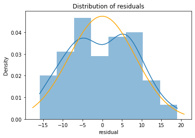
8.4. Histogram of residuals¶

Plotting residuals in Seaborn is straightforward: we simply pass the histplot() function the array of residuals from the regression model.

import seaborn as sns
sns.histplot(model_result.resid);

A slightly more useful approach for assessing normality is to compare the kernel density estimate with the curve for the corresponding normal curve. To do this, we generate the normal curve that has the same mean and standard deviation as our observed residual and plot it on top of our residual.

We use a Python trick to assign two values at once: the fit() function returns both the mean and the standard deviation of the best-fit normal distribution.

from scipy import stats
mu, std = stats.norm.fit(model_result.resid)
mu, std

(-1.283116008265812e-14, 8.418278511304978)

We can now re-plot the residuals as a kernel density plot and overlay the normal curve with the same mean and standard deviation:

import matplotlib.pyplot as plt
import numpy as np

fig, ax = plt.subplots()
# plot the residuals
sns.histplot(x=model_result.resid, ax=ax, stat="density", linewidth=0, kde=True)
ax.set(title="Distribution of residuals", xlabel="residual")

# plot corresponding normal curve
xmin, xmax = plt.xlim() # the maximum x values from the histogram above
x = np.linspace(xmin, xmax, 100) # generate some x values
p = stats.norm.pdf(x, mu, std) # calculate the y values for the normal curve
sns.lineplot(x=x, y=p, color="orange", ax=ax)
plt.show()

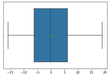
8.5. Boxplot of residuals¶

A boxplot is often better when the residuals are highly non-normal. Here we see a reasonable distribution with the mean close to the median (indicating symmetry).

sns.boxplot(x=model_result.resid, showmeans=True);

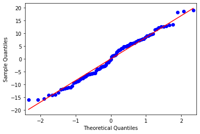
8.6. Q-Q plot¶

A Q-Q plot is a bit more specialized than a histogram or boxplot, so the easiest thing is to use the regression diagnostic plots provided by Statsmodels. How did I know Statsmodels has regression diagnostic plots? I Googled it. These plots are not as attractive as the Seaborn plots, but they are intended primarily for the data analyst. I think it is safe to assume that high-level decision makers will not be asking for Q-Q plots.

sm.qqplot(model_result.resid, line='s');

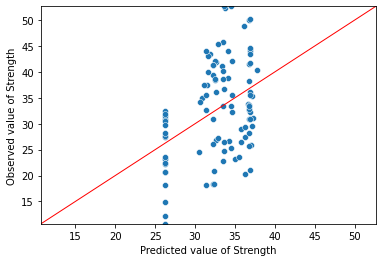
8.7. Fit plot¶

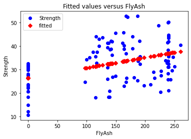
A fit plot shows predicted values of the response variable versus actual values of Y. If the linear regression model is perfect, the predicted values will exactly equal the observed values and all the data points in a predicted versus actual scatterplot will fall on the 45° diagonal.

The fit plot provided by Statsmodels is okay in the sense that it gives a rough sense of the quality of the model. Since the \(R^{2}\) of this model is only 0.165, it should come as no surprise that the fit model is not particularly good.

sm.graphics.plot_fit(model_result,1, vlines=False);

8.8. Fit plot in seaborn¶

As in R, creating a better fit plot is a bit more work. The central issue is that the observed and predicted axis must be identical for the reference line to be 45°. To achieve this, I do the following below:

Determine the min and max values for the observed values of Y
Predict values of Y
Create a plot showing the observed versus predicted values of Y. Save this to an object (in my case ax)
Modify the chart object so that the two axes share the same minimum and maximum values
Generate data on a 45° line and add the reference line to the plot

model_result.fittedvalues

    30.901424
    34.689565
    34.689565
    34.645517
    32.619302
         ...    
   36.808282
   36.843520
  36.830306
  36.843520
  36.103511
Length: 103, dtype: float64

Y_max = Y.max()
Y_min = Y.min()

ax = sns.scatterplot(x=model_result.fittedvalues, y=Y)
ax.set(ylim=(Y_min, Y_max))
ax.set(xlim=(Y_min, Y_max))
ax.set_xlabel("Predicted value of Strength")
ax.set_ylabel("Observed value of Strength")

X_ref = Y_ref = np.linspace(Y_min, Y_max, 100)
plt.plot(X_ref, Y_ref, color='red', linewidth=1)
plt.show()

7. Correlation and Scatterplots 9. Multiple Linear Regression

Basic Analytics in Python