Randomized Block Design
Read the section on Blocking Designs (pages 185-190) in Julian Faraway's Practical Regression and ANOVA using R (2002). This treatment of the topic is very concise and to the point, and gives the R commands and associated output and graphics. For supplemental reading you may look at Carl Schwarz's notes Chapter 7, which has good discussion of many of the issues surrounding randomized block experimental designs.The basic idea of blocking is to group the experimental units into blocks of similar units and carry out the treatment assignment separately within each block. With every treatment included at least once in every block the design is called a complete block design. When the assignment within each block is done with a completely randomized design, the design is called a randomized block design. In this section we will consider only randomized complete block designs.
Just as stratification in sampling can produce large gains in precidion of estimation, blocking in experiments can produce large gains in power. The reason is that often unit responses may be quite different in magnitude from one block to another, but the relative effects of different treatments are consistent from block to block. For example, in an agricultural experiment, fertility of soil may be much higher in the lower part of the field, so that yields there are overall higher than in the upper part of the field. However, the relative gain in yield from using one fertilizer versus another may be the same in both parts of the field. By separating the lower and upper parts of the field into blocks and assigning each treatment into each block, the comparisons of treatment effects can be made separately for the two blocks. Since there is much lower variation within each block, the denominator of the F statistic is smaller and, for a given size of treatment effect, the F statistic would tend to be higher with the blocked design.
Some learning goals for this section include being able to carry out the treatment assignment and the analysis of a randomized complete block experiment, understanding the underlying idea or reason for blocking so that you can identify situations in which blocking would be helpful, and understanding the assumptions on which the analysis is based.
Example: Effect of salinity on plant growth.
An experiment to investigate the effects of salinity in the soil on the growth of salt marsh plants is described by Carl Schwarz in Chapter 7 (p. 49) of his notes. There, the data from the randomized complete block experiment are analyzed using JMP software. Here, we will use R to do the same analysis.
There are six different salt treatments. The available experimental units are 24 plots. The assigned treatment is applied to the soil of a plot and at the end of the experiment the biomass for that plot is measured. The experimental units are gouped into four blocks of six plots each, based on geographic proximity, and the treatments are assigned completely at random within each block. Thus, each treatment occurs exactly once in each block.
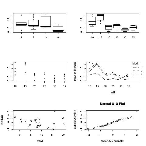
Diagnostic plots include boxplots of biomas for each block and for each treatment, a dot plot of the data for each treatment, an interaction plot showing the additive (or not) effect of the blocks, a plot of the residuals as a function of the fitted values, and a quantile-quantile plot to detect any departures of the residulas from normality.
Here are the R commands with the resulting output:
> saltmarsh <- read.table(file=url("http://www.stat.sfu.ca/~thompson/stat403-650/data/saltmarsh.txt"),header=T)
> names(saltmarsh)
[1] "Obs" "salt" "block" "biomass"
> saltmarsh
Obs salt block biomass
1 1 10 1 11.8
2 2 15 1 21.3
3 3 20 1 8.8
4 4 25 1 10.4
5 5 30 1 2.2
6 6 35 1 8.4
7 7 10 2 15.1
8 8 15 2 22.3
9 9 20 2 8.1
10 10 25 2 8.5
11 11 30 2 3.3
12 12 35 2 7.3
13 13 10 3 22.6
14 14 15 3 19.8
15 15 20 3 6.1
16 16 25 3 8.2
17 17 30 3 6.1
18 18 35 3 5.2
19 19 10 4 7.1
20 20 15 4 9.9
21 21 20 4 1.0
22 22 25 4 2.8
23 23 30 4 0.7
24 24 35 4 2.2
> attach(saltmarsh)
> class(salt)
[1] "factor"
> salt <- factor(salt)
> block <- factor(block)
> plot(biomass ~ block + salt)
Hit <Return> to see next plot: stripchart(biomass~salt,vert=T,pch=21)
Hit <Return> to see next plot: interaction.plot(salt,block,biomass)
> interaction.plot(block,salt,biomass)
> anova(lm(biomass ~ block + salt))
Analysis of Variance Table
Response: biomass
Df Sum Sq Mean Sq F value Pr(>F)
block 3 217.18 72.39 9.4152 0.0009603 ***
salt 5 680.81 136.16 17.7085 8.076e-06 ***
Residuals 15 115.34 7.69
---
Signif. codes: 0 ‘***’ 0.001 ‘**’ 0.01 ‘*’ 0.05 ‘.’ 0.1 ‘ ’ 1
The analysis of variance table line for salt (treatment) should be interpreted as testing for the effect of the treatment after fitting blocks into the model, that is, after the differences between blocks has been accounted for. The F statistic value of 17.7 is obtained by dividing the mean square for salt by the mean square residual. The effect of blocks is not tested for because blocks have not been randomly assigned, nor are they replicated.
> g <- lm(biomass ~ block + salt)
> anova(g)
Analysis of Variance Table
Response: biomass
Df Sum Sq Mean Sq F value Pr(>F)
block 3 217.18 72.39 9.4152 0.0009603 ***
salt 5 680.81 136.16 17.7085 8.076e-06 ***
Residuals 15 115.34 7.69
---
Signif. codes: 0 ‘***’ 0.001 ‘**’ 0.01 ‘*’ 0.05 ‘.’ 0.1 ‘ ’ 1
> tapply(biomass,salt,mean)
10 15 20 25 30 35
14.150 18.325 6.000 7.475 3.075 5.775
> plot(g$fitted, g$res, xlab="fitted",ylab="residuals")
> qqnorm(g$res)
----------------------------------------------------------------------------------------------------------------------------------------------
For convenience, first here are the commands used, printed without prompts or resulting output:
-----------------------------------------------------------------------------------------------------------------------------------------------
saltmarsh <- read.table(file="saltmarsh",header=T)
names(saltmarsh)
saltmarsh
attach(saltmarsh)
class(salt)
salt <- factor(salt)
block <- factor(block)
plot(biomass ~ block + salt)
stripchart(biomass~salt,vert=T,pch=21)
interaction.plot(salt,block,biomass)
interaction.plot(block,salt,biomass)
anova(lm(biomass ~ block + salt))
g <- lm(biomass ~ block + salt)
anova(g)
tapply(biomass,salt,mean)
plot(g$fitted, g$res, xlab="fitted",ylab="residuals")
qqnorm(g$res)
-----------------------------------------------------------------------------------------------------------------------------------------
The diagnostic plots can be put all together with the commands:
------------------------------------------------------------------------------------------------------------------------------------------
par(mfrow=c(3,2))
boxplot(biomass ~ block)
boxplot(biomass ~ salt)
stripchart(biomass~salt,vert=T,pch=21)
interaction.plot(salt,block,biomass)
plot(g$fitted, g$res, xlab="fitted",ylab="residuals")
qqnorm(g$res)
-----------------------------------------------------------------------------------------------------------------------------------------
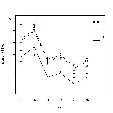
The following command shows the fitted model for the four blocks, where the assumption of no interaction forces the fitted values to constant distances apart, representing the assumed constant block effects. Next the actual data points are drawn, color coded by block. Finally, line segments representing the residuals are drawn connecting the data points to the corresponding fitted values.
interaction.plot(salt,block,g$fitted,ylim=c(-5,25))
points(salt,biomass,pch=21,bg=as.numeric(block))
segments(as.numeric(salt),g$fitted,as.numeric(salt),biomass)