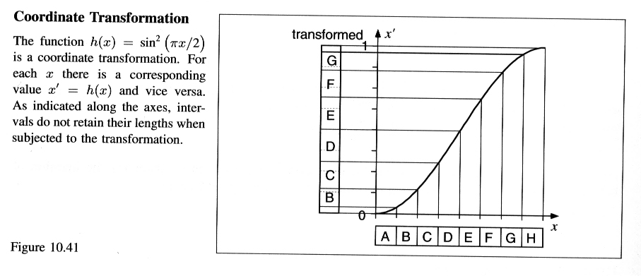
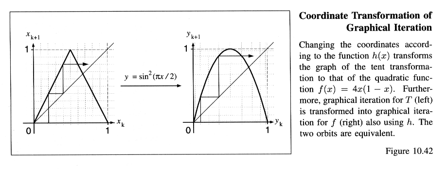
A very useful technique to study complicated dynamical systems is symbolic dynamics. We illustrate this method by studying the logistic equation 4x(1-x). First we introduce the Tent transformation T(x) = 2x if x<1/2; T(x) = 2 - 2x if x > 1/2. If you sketch the graphs of the Tent transformation and 4x(1-x) you will see that they are very similar; the graph of the Tent transformation is a linear (i.e., straight line) approximation of the graph of 4x(1-x); see Figure 10.42. The coordinate transformation y = h(x) = sin^2(x*pi/2) makes this explicit: T(x) is equivalent to 4y(1-y) where y = h(x). Thus, if {x, T(x), T^2(x), ... } is an orbit for T, then {h(x), h(T(x)), h(T^2(x)), ... } = {y, f(y), f^2(y), ... } is the equivalent orbit for f(x) = 4x(1-x), and visa versa (that is, starting with an orbit of f, we can find an orbit of T via the inverse transformation h^(-1)(y) = x); see equation (10.18) on page 561.
(
Larger view.)
So it is enough to study the orbits of T; this information will tell us
everything about the orbits of f(x) = 4x(1-x), which is what we are
interested in (see Figure 10.44). Now to study the orbits of T we make a
further "change
of coordinates", although this change of coordinates is between numbers
and sequences (h was a change of coordinates between numbers x
and y). Here we look at the binary representation of the Tent
transformation (page 556, 567). If we express numbers x by their binary
representation [x], then the tent transformation has a simple form; it
is shift left or shift-left-then-conjugate (note that the text uses the
term dual instead of conjugate).
We call this transformation
on sequences of 0's and 1's T~ ("T tilde"). So T~(.a_1 a_2 a_3 ...) =
.a_2 a_3 ... if a_1 = 0, or .a*_2 a*_3 ... if a_1 = 1, where a* is the
conjugate of a . T~ replicates
the action of T, but on the binary representation of numbers instead of on
the numbers themselves; T~([x]) = [T(x)], and so (T~)^n([x]) = [T^n(x)].
Thus, we can study the behavior of orbits of T by studying the behavior of
orbits of T~.
The simple action of T~ on sequences (of 0's and 1's) makes it easy to
completely describe the types of orbits T~ has. Thus, we will be able to
completely describe the orbits of T, and so the orbits of f(x) = 4x(1-x).
Of the many questions we could ask about orbits of T, a few would be; Does T have periodic points? Does T have an ergodic orbit? How are the periodic and ergodic points of T distributed (eg. are they dense)? We showed in class (see also pages 552 - 559) how these questions could be answered fairly easily by considering the map T~ on sequences first, and then translating these results to T by converting the sequence .a_1 a_2 a_3 ... into a number x (so [x] = a_1 a_2 a_3 ... ). Then, we convert these into answers for f(x) = 4x(1-x) via the coordinate transformation h(x).
As a result, we can say quite a bit about the logistic equation f(x) = 4x(1-x). We can prove sensitive dependence on initial conditions and mixing, two of the hall marks of chaos (the other being dense periodic points; see below). We can prove that there are periodic orbits of all periods, that the set of periodic points is dense in [0,1], and that the set of ergodic points is also dense in [0,1]. What we didn't prove is that the "length" of the set of periodic points (i.e., if you put all the periodic points together and measured the length of that set) is 0, while the "length" of the set of ergodic points is 1. Another way of putting this is that if you randomly choose a number from [0,1], with probability 0 it will be a periodic point (i.e., will generate a periodic orbit under iteration by f), while with probability 1 the number will be an ergodic point of f (i.e., its orbit will be ergodic). Note that a periodic orbit is the antithesis of an ergodic orbit ( a periodic orbit only visits a few points in the interval [0,1], while an ergodic orbit visits "nearly every" point in [0,1]; one is completely 'orderly' while the other is completely 'random'), but the two types are intimately intertwined ("There is order within chaos").
A final remark. If instead we are considering the logistic equation ax(1-x) for a not equal to 4, we have to find another way to represent the dynamics 'symbolically'. However, it is not always possible to find a symbolic dynamics. In the case when a is greater or equal to 4 it is always possible to represent the dynamics as a shift and shift-and-congugate on sequences of two symbols (say, 0 and 1). You can find out more about this by looking at the book "A First Course in Discrete Dynamical Systems" by R. A. Holmgren Chapter 11 for example. For a more general discussion on symbolic dynamics, including the "Smale Horseshoe" (a paradigm for complicated dynamics), see Chapter 5 of "Nonlinear Oscillations, Dynamical Systems, and Bifurcations of Vector Fields" by J. Guckenheimer and P. Holmes.
The logistic equation 4x(1-x) is chaotic. In particular, it is extremely sensitive to errors (errors approximately double with each iteration). We have seen computations of orbits of up to 100,000 iterations using a computer. Now, a computer can not represent all numbers exactly. For example, if your computer can only retain 14 decimal places, then only those numbers that have decimal representations of 14 or less digits can be represented exactly (I'm considering numbers in [0,1]). In particular, irrational numbers can not be represented on a computer (all computations are with rational numbers, and only those that have decimal expansions of 14 digits or less).
When the computer iterates f(x) it may be introducing an error (of the size 10^(-14) or so) at each iteration (unless f(x) is exactly representable on the machine). These errors grow very quickly, so what are these computations telling us about the exact dynamics? Can we say anything at all about the exact dynamics based on computer simulations? For certain dynamical systems, of which 4x(1-x) is one, it turns out that even if our computations may be making errors at each step in the iteration of an orbit, there is still an orbit of the exact dynamics that is close to the computed orbit. This is the Shadowing Lemma (an exact orbit "shadows" the computed orbit). So even if our computer simulations of orbits are not exact orbits at all, there is an exact orbit close to the one we compute. So for example, if we compute a histogram of an orbit and it appears to be ergodic (i.e., the histogram fills the interval [0,1]), then we can conclude, by the Shadowing Lemma, that there is an ergodic orbit of the exact dynamics.
Here is a version of the Shadowing Lemma, taken from the book "Nonlinear
Oscillations, Dynamical Systems, and Bifurcations of Vector Fields" by J.
Guckenheimer and P. Holmes, page 251:
For every b > 0 there is an a > 0 such that every a-pseudo orbit
is b-shadowed by an exact orbit.
Here, an "a-pseudo orbit" is a computed orbit that may have an error of
size a at each iteration (eg. computer simulation), while "b-shadowed"
means there is an exact orbit that is within a distance b of the computed
orbit at each iteration. Thus, we can be assured that an exact orbit is
very close to the computed one by making the errors at each iteration
small enough. The theorem applies to "hyperbolic invariant sets" so you
need to verify this for your particular dynamical system.
In general, computer simulation of dynamical systems (discrete or continuous) is tricky business. Even if the computations are very accurate (i.e., errors are small), the nature of the underlying exact dynamics may cause the computations to "run away" from the exact dynamics. From another point of view, there are a lot of papers published in the journals about computer simulations of chaotic systems. Now, establishing a theoretical proof that a dynamical system is chaotic (sensitive dependence, mixing, dense periodic orbits) is one thing, but using computer experiments to conclude a system is chaotic is quite another. Edward Lorenz (who discovered the 'Lorenz Attractor') wrote an article on "Computational Chaos" (Physica D (1989) page 299-317) in which he describes how an otherwise non-chaotic dynamical system can appear to be chaotic if one is not careful with the way the computations are carried out.