 Figure 11.5 is the final-state diagram for the logistic
function. Go
here
for a larger view.
Figure 11.5 is the final-state diagram for the logistic
function. Go
here
for a larger view.
Graphical iteration (or graphical analysis as it is sometimes called) is a way to study orbits of a function f graphically by following the orbit as it moves along the diagonal line y = x which is drawn along with the graph of the function. For example, fixed points p of f are the x-coordinates of the points of intersection of the graph of f and the line y = x; f(x) = x. Notice that the orbit of a fixed point p is {p, p, p, ... }.
The next thing to ask is what is the stability of the fixed point. We say that a fixed point is stable if orbits that start nearby the fixed point converge to the fixed point as n tends to infinity ( x_n = f^n(x_0) ). We call the fixed point unstable if at least one nearby point has an orbit that does not converge to the fixed point. The stability of a fixed point refers to whether it is stable or not. Note that a fixed point need not be stable or unstable. Consider the function f(x) = 2 - x. Here the fixed point is p = 1. Now, f^2(x) = f(f(x)) = 2 - ( 2 - x ) = x, so that every orbit of f is periodic of period 2. Thus, the orbits of points near p neither converge to p nor move away from p. We call this kind of stability neutral stability.
It is easy to determine the stability of a fixed point using graphical analysis (see the handout). From that we see that the stability of a fixed point could also be determined analytically; the fixed point p is stable if if | f '(p) | < 1 and is unstable if | f '(p) | > 1. In the case | f '(p) | = 1, the fixed point could be either stable, unstable, or neutral. So in this case one has to make a careful sketch of the graph of f near the fixed point to determine the stability. All one needs to know in order to determine the stability of a fixed point p from graphical analysis is how the graph of f lies with respect to the diagonal line y = x near p (see the figures in the handout).
Periodic orbits of (prime) period greater than one are not easy to detect graphically with f. Here we should apply graphical analysis to f^k if we want to study periodic points of f of period k. So we would first look for fixed points of f^k, i.e., we would solve f^k(x) = x (keep in mind our notation; f^k denotes the k-fold convolution of f, not the product of f with itself k times). Graphically, these would be the x-coordinates of points of intersection between the graph of f^k and the line y = x. Using graphical analysis we could then determine the stability of these fixed points of f^k. We call a periodic point q stable if | (f^k(q))' | < 1 and unstable if | (f^k(q) )'| > 1. The stability of a periodic point q of f of period k is then just the stability of the fixed point q of f^k. So if q is a stable periodic point of f of period k, then the orbits starting at points near q will converge to the periodic orbit of q. And if q is unstable then at least one nearby point will have an orbit that does not converge to the periodic orbit of q.If we are considering a function f_a(x) that depends on a parameter a, then since the graph of f will (perhaps) change as the parameter a changes, we expect that the periodic points of f will also change with a. Change here could mean that the periodic point changes location as a changes and also its stability could change. In addition, a periodic point can appear or disappear as a changes. When the qualitative behavior of the orbits of f_a changes at a certain parameter value, say a = b_1, then we call that value of a a bifurcation point of f_a and say that "f_a undergoes a bifurcation at a = b_1" (consider the final-state diagram of f_a discussed below; it undergoes a drastic change at the bifurcation points of f_a). For example, if f_a(x) = ax(1-x), the logistic function, then f_a undergoes a bifurcation at a = 3 because the fixed point of f_a changes from stable to unstable at a = 3. That's enough to call a = 3 a bifurcation point, but in addition a period two orbit appears, which also changes the qualitative behavior of the orbits of f_a.
We can understand this "period doubling" bifurcation of the logistic function at a = 3 from graphical analysis. If you look at Figure 11.18 you see how two new fixed points of (f_a)^2 appear as a increases through the value 3. Notice too that these two new points "come out of" the fixed point p of f_a. If we continue to increase a further, these period two points will undergo a bifurcation; they will change from stable to unstable and just when they become unstable a period 4 orbit appears. An infinite sequence of such period doublings occurs as a increases, but the distance (in a) between successive bifurcations decreases geometrically, so that these points of bifurcation accumulate at the value 3.5699.... . This is described on pages 608 - 612.
A bifurcation diagram is the plot of the locations of the fixed
points versus the parameter value a. Figure 11.17 shows part of the
bifurcation diagram for the logistic function. Here one solves the
equation f_a(p_a) = p_a for the fixed points of
f_a; p_a = (a-1)/a and 0.
The curves (a-1)/a and 0 are drawn on the
bifurcation diagram. Then one
solves the equation (f_a(q_a))^2 = q_a
for the period 2 points. The curves
q_a are then drawn on the bifurcation diagram
(there are two such curves
for period 2 because there are 2 period 2 points). In general, bifurcation
diagrams are diffucult to draw because one has to solve the equations
(f_a(x))^k = x (and then plot the curves x as a function of
a). A similar
diagram that can be drawn using computer generated orbits of f_a is
the final-state diagram (see page 586,587).
Here one plots the 'final state' of an orbit {x_n} of f_a;
say x_101 to x_200. If the
orbit is periodic, or is converging to a periodic orbit, the final state
will be that orbit. If a periodic orbit attracts (essentially) all the
orbits no matter where they begin, then the final state will be the same
no matter where the orbit starts. Now change a
a little and plot x_101 to
x_200, etc., for a range of a values. What one sees then are the
stable periodic orbits. If f_a happens not to have any stable
periodic orbits, then the final state of an orbit will be points spread out
over a portion of the interval [0,1] instead of being concentrated in just a
few points.
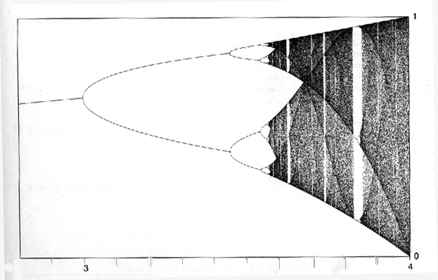
Figure 11.5 is the final-state diagram for the logistic
function. Go
here
for a larger view.
The final-state diagram of the logistic function for parameter values a between 1 and 4 has remarkable and complex patterns. For a greater than 1 we see the period doubling bifurcations culminating at the point 3.699... , and as a is increased further a very different pattern appears. This pattern continues to evolve and change as a increases. Bands of chaotic behavior open up while occassionally periodic 'windows' of stable orbits appear. Finally, at a = 4, there is chaotic behavior across the entire interval [0,1]. There are many unanswered questions about the structure of this diagram that are topics of current mathematical research (see for instance the book "Iterated Maps on the Interval as Dynamical Systems", by P. Collett and J-P Eckmann).
Universality (see pages 610-618)There are infinitely many functions g_a that go through a series of period doubling bifurcations in a simialr way as the logistic function does as the parameter a changes. In fact, if g(x) is a continuous function that has a single maximum in [0,1] and is stricly increasing or decreasing on either side of the maximum, then the function g_a(x) = ag(x) goes through a sequence of period doubling bifurcations as a increases. Now, this is not so surprising when you think about the shapes of the graphs of (g_a)^k; since g_a is similar to f_a, (g_a)^k goes through similar changes as a increases, so we can see how new periodic points come into being just as we saw for the logistic function (above). What is remarkable is that the rate at which these period doubling bifurcations occur is the same for all functions! More precisely, if d_k = b_(k+1) - b_k (where b_k are the points of period doublings for the logistic equation) and if c_k = e_(k+1) - e_k where e_k are the points of period doubling bifurcations of g_a, then the limit as k tends to infinity of the ratios (d_k/d_(k+1)) and (e_k/e_(k+1)) are the same! (precisely, 4.6692...) That this is true for such a wide variety of functions was completely unexpected when it was discovered in the 1970's. It was Mitchell Feigenbaum who explained this using the Renormalization Group method from theoretical physics in 1977, and the result has come to be known as 'universality'. This indicates that there are universal mechanisms that produce chaos from ordered systems, and a study of these mechanisms is one of the current areas of research in chaos theory.
As another feature of universality, look at the final state diagram of the function g_a(x) = ax^2(sin(pi*x)); Figure 11.23. It looks remarkably like the final state diagram of the logistic function. In fact, the final-state diagrams of many very different dynamical systems look a lot like the final state diagram of the logistic function (see for example Figures 12.15 and 12.30).
For a brief discussion of renormalization, see pages 470-474 in the text. For a general introduction to the renormalization group method in statistical physics, see the article "Critical point phenomena: universal physics at large length scales", by A. Bruce and D. Wallace, in the book The New Physics edited by P. Davies. For even more information about the renormalization group and critical phenomena in physics, I'd recommend the book "Quantum and Statistical Field Theory", by Michel Le Bellac (Oxford, 1998,1991). The universality Feigenbaum discovered with the functions g_a as the parameter a approaches the limiting value b_infinity is analogous to the universality physicists discovered in the behavior of fluids and solids near the 'critical point' (ie., near a phase transition). The limiting value b_infinity for the functions g_a is analogous to the critical temperature T_c where the phase transition occurs in these physical systems (so we can say that the functions g_a undergo a 'phase transition' as the parameter value a passes through the limiting value b_infinity; the very different appearance of the final state diagram for g_a on either side of b_infinity shows the two 'states' of g_a - on one side g_a is very ordered and on the other side g_a is chaotic). In the same book The New Physics is an article "Physics of far-from-equilibrium systems and self-organization" by G. Nicolis which also mentions the renormalization group method but also discusses nonlinear dynamical systems in physics, chemistry and biology which exhibit chaos, bifurcations, strange attractors, etc.
Charkovsky's Theorem (see pages 638,639)In 1964 A. N. Charkovsky proved a remarkable theorem about the periodic points of functions. To state the theorem we have to introduce a new ordering of the natural numbers, the Charkovsky Ordering. The ordering is as follows. 3 >> 5 >> 7 >> 9 >> ... >> (2)3 >> (2)5 >> (2)7 >> ... >> (2^2)3 >> (2^2)5 >> (2^2)7 >> ... >> (2^3)3 >> (2^3)5 >> ... ... >> (2^n)3 >> (2^n)5 >> ... ... >> 2^5 >> 2^4 >> 2^3 >> 2^2 >> 2 >> 1. The ordering starts with 3 and proceeds through the odd numbers, then through the numbers of the form (2)(odd), and then through the numbers of the form (2^2)(odd) etc, and finally through the numbers of the form 2^m in decreasing order, ending with 1. You can check that every natural number is listed here, and only once. We say "a precedes b" in this ordering if a comes before b in the Charkvsky ordering (i.e, a >> b). In this ordering, 3 is the largest number and 1 is the smallest. Also, every odd number is before any even number. To determine where a number A sits in the Charkovsky ordering you have to write it as (2^k)(odd). For example, 27 = (2^0)(27), 32 = (2^5)(1) and 48 = (2^4)(3). Thus, 27 preceeds 48 and 48 preceeds 32 in the Charkovsky ordering (note that the Charkovsky ordering does not always agree with the usual a < b ordering of the natural numbers). Charkovsky's Theorem is: If f is a continuous function that transforms an interval I onto itself (i.e., f(I) is contained in I), and if f has a periodic point of period k, then f has a periodic point of period m for every m such that k >> m in the Charkovsky ordering.
One of the many consequences of Charkovsky's Theorem is that if f has a period 3 point, then f has a periodic point of each (prime) period. So if you know f has a period 3 orbit then you know that there is a periodic orbit of period k for every k. This is sometimes referred to as "period 3 implies chaos" because the existence of infinitely many periodic orbits sometimes implies that the dynamical system is chaotic (see page 133 of Devaney's book listed below). Using the example above, if f has a periodic point of period 27, then f has a periodic point of period 48, and if f has a periodic point of period 48 then f has a periodic point of period 32. Furthermore, if you look closely at the final state diagram for the logistic function (Figure 11.5 or 11.41) you will see a 'period 3 window' near a = 3.83 (there are only 3 points in the 'final state' of an orbit at that parameter value). Now, every computation of an orbit of the logistic function for a = 3.83 will give the final state as the same three points (the period 3 orbit). Now, from Charkovsky's Theorem there are infinitely many periodic points of the logistic function for a = 3.83 (because 3 is the first number in the Charkovsky ordering). How come we never see these orbits with the computer? For the simple reason that they are all unstable periodic orbits; they don't attract any nearby points. Keep in mind too that the computer introduces small errors at each iteration, so even if you started the computation off on one of these unstable periodic points, the computed orbit would quickly move away from this periodic orbit (and instead converge to the stable period 3 orbit).
For an idea of the proof of Charkovsky's Theorem see Chapter 11 of R. Devaney's book, "A First Course in Chaotic Dynamical Systems".