Methods

Research Question:

What are the playability scores of neighborhoods in the Grandview-Woodland and Lonsdale neighbourhoods?

Data Digitization and Categorization:

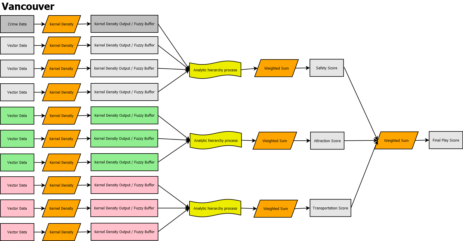
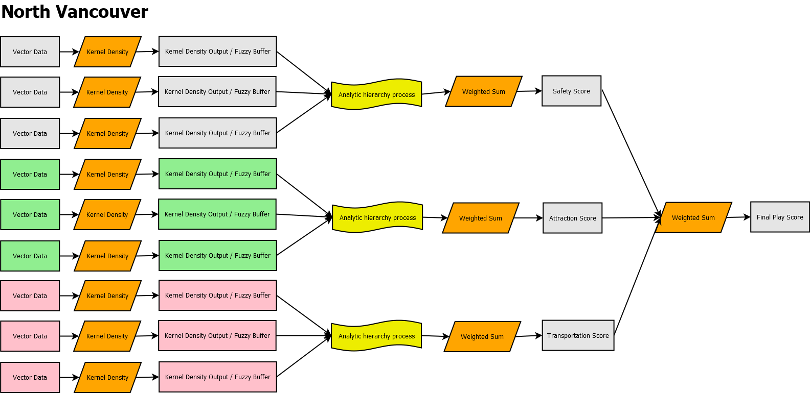
To assess playability in the two study areas, a Multi-Criteria Analysis (MCA) was chosen. Figure two (above) illustrates the workflow necessary to conduct a MCA which include preparing and weighing various datasets. Interview and survey data from both subjects and parents were analyzed to chose relevant datasets of use. A three-tiered approach of transportation, safety and attraction was used to determine playability which was reflective of what the subjects and parents determined was important in a playable neighbourhood. Available datasets were analyzed and assigned to one of three categories. Since there was a surplus of data, it was ultimately unfeasible and ineffective to have all datasets incorporated into the analysis, datasets believed to be more important based on literature reviews, common knowledge and interview/survey data were given priority and assigned to their respective category. Datasets that were incomplete or missing was created/digitized using digital audits by way of Google Street View and ArcMap. To ensure accuracy, physical site audits were also conducted. Once all data sets were assembled, their accuracy was compared to known spatial data values and any deficiencies were addressed.

The safety aspect of playability was first to be determined and would be used to derive an overall playability score. The reasoning was safer neighborhoods would reassure parents in allowing children to play outside and give said children a sense of comfort in encouraging outdoor physical play in the community. It was determined that safety would be based on physical infrastructures such as traffic calming measures, as compared to non-spatial perceptions of safety which may vary from person to person and are difficult to measure objectively and spatially. Traffic calming measures was used to gauge the road safety of neighborhoods, which included data sets on streets, crosswalks, four way stops, speed bumps and roundabouts into this portion of the analysis. Collectively, all datasets deemed as related to each of these safety factors will be used to develop a safety index of neighborhoods and will have an influence on the final playability score.

The attractiveness of a play environment for 10-13-year-old children was determined next. Appealing play spaces for the target audience is important, as children will be more encouraged to spend time outside in their communities if there are suitable places to utilize for play. We have a collection of data which are known to be popularly occupied play spaces to the target demographic, based on interview data. We have also incorporated data sets that have value as potential play spots based on our own knowledge and literature. Attractive play areas to kids can include: trails, parks, community centers, schools, roundabouts, bikeways, playgrounds, sports fields and libraries.

Finally, the transportation aspect of playability was determined. For the target demographic, bikeability and walkability are the variables that will be included into the transportation score. Based on trends seen in interviews, most 10-13-year-old children tend to either walk or bike to areas they play and are less likely to take public transportation without a parent. The higher the transportation rating of a neighborhood, the more play is encouraged, as easy accessibility by foot is an incentive for children to utilize available play environments. The datasets that can be used to infer the transportation rating of an area are; sidewalks, bikeways, trails and crosswalks. The last step of our playability analysis was to combine the safety, transportation and attraction scores of each neighborhood for a playability analysis that considers all the chosen variables.

Kernel Density Analysis:

Kernel density outputs were then created for each variable included in the playability analysis separately. Kernel density calculates “a magnitude per-unit area from point or polyline features, using a kernel function to fit a smoothly tapered surface to each point or polygon” (ESRI, 2017). By preforming a kernel density analysis for each variable, we were able to visualize the density of features and essentially create Euclidean fuzzy buffers around the features based on our chosen parameters. Euclidean distance analysis was chosen over a network distance as the target demographic typically does not strictly follow pathways, roads or bikeways (common network distance methods), as they travel by foot or bike and can move more fluidly throughout their neighborhoods. It was also evident from interview data that children liked to make use of alleyways, shortcuts and unofficial greenspaces when traveling and would be difficult to represent as a Manhattan (network) style distance analysis.

A kernel destiny model needs parameters to create a distance analysis such as; features (the point, line and polygon data for which to calculate the density), cell size (the resolution of the raster output, a 15m resolution was decided upon to completed the analysis at a reasonable time and sharpness), search radius (the distance which the density is calculated within) and units (m2 was chosen, as it was most appropriate at the neighborhood level). Parameters for the search radii varied for each section of the playability analysis, as using one general radius would not be as true representation of reality for all variables considered. However, it was decided that it made the most sense if the variables contained within the attraction, transportation and safety analyses had a uniform radius.

For the attraction kernel density analysis, a search radius of 1 km was chosen as ideal. This was determined because typically the furthest distance that children in interviews would play from home was a ten-minute walk and the majority played even closer to home than that. The average walking speed is 0.6 miles or 1 km per hour and since 10-13-year old are not small children, they fit into the average walking speed assumption and would cover a distance of about 1 km in 10 minutes (Barkley & Lepp, 1). The search radius for transportation was a little different than for attractive play places because the transportation data consists of infrastructure such as sidewalks, which are expected to be more accessible in an ideal neighborhood, therefore closer together in distance. We decided that a 2-minute walk to a sidewalk or crosswalk was appropriate, as the distance was reasonably attainable, and this would be the equivalent of a 0.2 km radius. The safety analysis once again consisted of mostly infrastructure, so we believed that the radius should be smaller to identify neighborhoods that had a high density of traffic calming measures from those that did not. Coming up with an actual distance was difficult, so a trial and error process was needed. First, areas that had a high density of safety infrastructure were identified and the average distance between the safety infrastructure was our “ideal” distance and incorporated into our search radius for safety (100 m).

Weighted Sum Analysis:

The weighted sum analysis is a multi-criteria evaluation tool used in ArcMap to apply weights to variables in our safety, transportation and attraction playability analysis to assign a ranking or score to each neighborhood. Weighted sum works by overlaying multiple raster layers and multiplying each one by a given weight (any negative or positive decimal) to sum them together (ESRI, 2011). For each of the three categories, weights were determined separately to properly rank variables that correspond with results from interview data and meta-analysis. The variables that were included in the attractiveness analysis were all assigned an equal weight. This is because density of the “attractive” play places was more important than the actual type of play place, therefore areas that had a higher number of attractive play places would earn a higher playability score than areas that had less. A higher density of attractive places also meant that individual children had a greater chance of finding a play place close to their neighborhood that suits their needs, as they have a greater variety to choose from. We believe that it was a subjective concept that certain play places are more attractive than others, as opinions vastly differ between children. For example, while reading interview data we came across children who preferred libraries over parks and vice versa. Therefore, attractiveness is not weighted and is purely based on density. The same concept applies for transportation scoring, as an equal weight was also applied for our four-chosen transportation related variables. Once again, density of sidewalks, bikeways, crosswalks and trails was more important than ranking which variables are more useful to children, as interview data suggested that opinions and rankings were highly based on individual opinions.

For the safety score, weights were needed, as certain variables increased safety, while other variables decreased safety. Literature also suggested that certain variables were deserving of a higher safety rating than others. For example, a study at the Institute of Transport Economics in Norway studied 44 other papers regarding converting intersections to roundabouts and it was concluded that roundabouts were able to reduce fatal accidents by 65% and reduce injury by 40% (Elvik, 364). An analytical hierarchy process was used to formalize the weighting scheme of our safety score. Factors that are generally agreed upon to increase safety are traffic calming measures such as: crosswalks, four way stops and roundabouts. On the other hand, intersections, crime and busy roads have been linked to increased chance of injury, reducing safety. The analytical hierarchy process (AHP) aids with the complex decision making associated with ranking the variables and was used to formally quantify weights for our safety model. The first step in conducting our AHP was computing the matrix of option scores. To do so, a pairwise comparison matrix in the format of an n x n matrix, where n is the number of criteria (Saaty, 85). The importance of the criterion is then ranked on a numerical scale from 0 to 1, with 1 being that the first criteria is much more important than the second and 0 being that they are equal. After ranking is complete, the criteria weight vector is calculated by averaging values in each row (Saaty, 90). The next step of the AHP is creating a matrix of option scores in an m x n format. The options are then weighted against one another and if the option is given a score of >1, then the first option is greater than the second, while a score of <1 indicates the first option is worse than the second and if given a score of 1 the options are equal. The last step of the AHP was to multiply the numbers derived from step 1 (weight vector), with step 2 (score matrix) to derive a global score for each variable (Saaty, 94). These three steps were followed for the safety variables to assign them numerical values that express their ranking in importance to safety. Traffic calming (0.331), speed humps (0.231), crosswalks (0.157) and roundabouts (0.106) were assigned the highest weights as they were the most important factors in positively impacting safety. Four-way stops were assigned a lower weight (0.071), because even though they are a traffic calming measure, they often are the scene of accidents with pedestrians. Lastly, intersections (0.048) and streets (0.033) were assigned low weights because there is consensus that they are often the places were pedestrian injuries and fatalities occur.