Chapter Contents
Previous
Next
|
Chapter Contents |
Previous |
Next |
| QQPLOT Statement |
| See CAPQQ2 in the SAS/QC Sample Library |
The three-parameter lognormal distribution depends
on a threshold parameter ![]() , a
scale parameter
, a
scale parameter ![]() , and a shape parameter
, and a shape parameter ![]() .You can estimate
.You can estimate
![]() from a series of lognormal Q-Q plots with different
values of
from a series of lognormal Q-Q plots with different
values of ![]() .The estimate is the value of
.The estimate is the value of ![]() that
linearizes the point pattern. You can then
estimate the threshold and scale parameters from the
intercept and slope of the point pattern. The following
statements create the series of plots
in Output 10.2.1 through Output 10.2.3 for
that
linearizes the point pattern. You can then
estimate the threshold and scale parameters from the
intercept and slope of the point pattern. The following
statements create the series of plots
in Output 10.2.1 through Output 10.2.3 for
![]() values of 0.2, 0.5, and 0.8:
values of 0.2, 0.5, and 0.8:
   title 'Lognormal Q-Q Plot for Diameters';
   proc capability data=measures noprint;
      qqplot diameter / lognormal(sigma=0.2 0.5 0.8)
                        square
                        cframe = ligr;
   run;
Output 10.2.1: Lognormal Quantile-Quantile Plot (

|

|
Output 10.2.3: Lognormal Quantile-Quantile Plot (

|
The plot in Output 10.2.2 displays the most linear
point pattern, indicating that the lognormal distribution
with ![]() provides a reasonable fit for the data
distribution.
provides a reasonable fit for the data
distribution.
Data with this particular lognormal distribution have the density function
The points in the plot fall on or near the line with intercept
| See CAPQQ2 in the SAS/QC Sample Library |
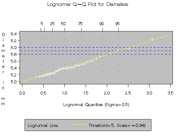
You can use a Q-Q plot to estimate percentiles such as the 95 th percentile of the lognormal distribution.*
The point pattern in Output 10.2.2 has a slope of
approximately 0.39 and an intercept of 5.
The following statements
reproduce this plot, adding a lognormal
reference line with this slope and intercept.
The result is shown in Output 10.2.4.
   title 'Lognormal Q-Q Plot for Diameters';
   legend1 frame cframe=ligr cborder=black position=center;
   proc capability data=measures noprint;
      qqplot diameter / lognormal(sigma=0.5 theta=5 slope=0.39
                                  color=yellow)
                        pctlaxis(grid lgrid=35)
                        vref  = 5.8 5.9 6.0
                        cvref = blue
                        cframe = ligr
                        legend=legend1;
   run;
Output 10.2.4: Lognormal Q-Q Plot Identifying Percentiles

|
Alternatively, you can compute this percentile from
the estimated lognormal parameters.
The ![]() percentile of the lognormal distribution is
percentile of the lognormal distribution is


| See CAPQQ2 in the SAS/QC Sample Library |
If a known threshold parameter is available, you can construct a two-parameter lognormal Q-Q plot by subtracting the threshold from the data and requesting a normal Q-Q plot. The following statements create this plot for DIAMETER, assuming a known threshold of five:
   data measures;
      set measures;
      label logdiam = 'log(Diameter-5)';
      logdiam = log( diameter - 5 );
   title 'Two-Parameter Lognormal Q-Q Plot for Diameters';
   legend1 frame cframe=ligr cborder=black position=center;
   proc capability data=measures noprint;
      qqplot logdiam / normal(mu=est sigma=est color=yellow)
                       vaxis=axis1
                       square
                       cframe=ligr
                       legend=legend1;
      axis1 label=(a=90 r=0);
   run;
Output 10.2.5: Two-Parameter Lognormal Q-Q Plot for Diameters

|
|
Chapter Contents |
Previous |
Next |
Top |
Copyright © 1999 by SAS Institute Inc., Cary, NC, USA. All rights reserved.