Example 29.2: Creating Two-Way Comparative Pareto Charts

Details and Examples

Example 29.2: Creating Two-Way Comparative Pareto Charts

See PARETO9 in the SAS/QC Sample Library

During the manufacture of a MOS capacitor, different cleaning processes were used by two manufacturing systems operating in parallel. Process A used a standard cleaning solution, while Process B used a different cleaning mixture that contained less particulate matter. The failure causes observed with each process for five consecutive days were recorded and saved in a SAS data set called FAILURE4.

   data failure4;
      label cause = 'Cause of Failure' ;
      input process $ 1-9 day $ 13-19 cause $ 23-36 counts 40-41;
      datalines;
   Process A   March 1   Contamination    15
   Process A   March 1   Corrosion         2
   Process A   March 1   Doping            1
   Process A   March 1   Metallization     2
   Process A   March 1   Miscellaneous     3
   Process A   March 1   Oxide Defect      8
   Process A   March 1   Silicon Defect    1
   Process A   March 2   Contamination    16
   Process A   March 2   Corrosion         3
   Process A   March 2   Doping            1
   Process A   March 2   Metallization     3
   Process A   March 2   Miscellaneous     1
   Process A   March 2   Oxide Defect      9
   Process A   March 2   Silicon Defect    2
   Process A   March 3   Contamination    20
   Process A   March 3   Corrosion         1
   Process A   March 3   Doping            1
   Process A   March 3   Metallization     0
   Process A   March 3   Miscellaneous     3
   Process A   March 3   Oxide Defect      7
   Process A   March 3   Silicon Defect    2
   Process A   March 4   Contamination    12
   Process A   March 4   Corrosion         1
   Process A   March 4   Doping            1
   Process A   March 4   Metallization     0
   Process A   March 4   Miscellaneous     0
   Process A   March 4   Oxide Defect     10
   Process A   March 4   Silicon Defect    1
   Process A   March 5   Contamination    23
   Process A   March 5   Corrosion         1
   Process A   March 5   Doping            1
   Process A   March 5   Metallization     0
   Process A   March 5   Miscellaneous     1
   Process A   March 5   Oxide Defect      8
   Process A   March 5   Silicon Defect    2
   Process B   March 1   Contamination     8
   Process B   March 1   Corrosion         2
   Process B   March 1   Doping            1
   Process B   March 1   Metallization     4
   Process B   March 1   Miscellaneous     2
   Process B   March 1   Oxide Defect     10
   Process B   March 1   Silicon Defect    3
   Process B   March 2   Contamination     9
   Process B   March 2   Corrosion         0
   Process B   March 2   Doping            1
   Process B   March 2   Metallization     2
   Process B   March 2   Miscellaneous     4
   Process B   March 2   Oxide Defect      9
   Process B   March 2   Silicon Defect    2
   Process B   March 3   Contamination     4
   Process B   March 3   Corrosion         1
   Process B   March 3   Doping            1
   Process B   March 3   Metallization     0
   Process B   March 3   Miscellaneous     0
   Process B   March 3   Oxide Defect     10
   Process B   March 3   Silicon Defect    1
   Process B   March 4   Contamination     2
   Process B   March 4   Corrosion         2
   Process B   March 4   Doping            1
   Process B   March 4   Metallization     0
   Process B   March 4   Miscellaneous     3
   Process B   March 4   Oxide Defect      7
   Process B   March 4   Silicon Defect    1
   Process B   March 5   Contamination     1
   Process B   March 5   Corrosion         3
   Process B   March 5   Doping            1
   Process B   March 5   Metallization     0
   Process B   March 5   Miscellaneous     1
   Process B   March 5   Oxide Defect      8
   Process B   March 5   Silicon Defect    2
   ;

In addition to the process variable CAUSE, there are two classification variables in this data set: PROCESS and DAY. The variable COUNTS is a frequency variable.

This example creates a series of displays that progressively use more of the classification information.

Basic Pareto Chart

The first display, created with the following statements, analyzes the process variable without taking into account the classification variables.

   title 'Pareto Analysis of Capacitor Failures' ;
   proc pareto data=failure4;
      vbar cause / freq     = counts
                   last     = 'Miscellaneous'
                   scale    = count
                   anchor   = bl
                   cframe   = ligr
                   cbars    = vigb
                   cconnect = salmon
                   nlegend ;
   run;

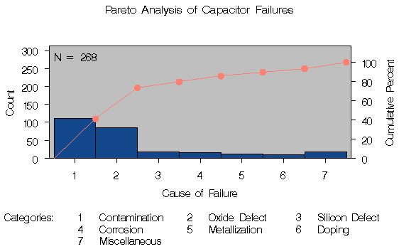
The chart, shown in Output 29.2.1, indicates that contamination is the most frequently occurring problem.

Output 29.2.1: Pareto Analysis without Classification Variables

The color and pattern for the bars are specified with the CBARS= and PBARS= options. The pattern M5X45 is a particular type of crosshatching (refer to SAS/GRAPH Software: Reference for a pattern selection guide). If you specify a color but not a pattern, the bars are filled with a solid color.

The option ANCHOR=BL anchors the cumulative percent curve at the bottom left (BL) of the first bar. The NLEGEND option adds a sample size legend.

One-Way Comparative Pareto Chart for PROCESS

The following statements specify PROCESS as a classification variable to create the comparative Pareto chart displayed in Output 29.2.2:

   title 'Pareto Analysis by Cleaning Process' ;
   proc pareto data=failure4;
      vbar cause / class       = process
                   freq        = counts
                   last        = 'Miscellaneous'
                   scale       = count
                   catleglabel = 'Failure Causes:'
                   intertile   = 1.0
                   cframe      = ligr
                   cbars       = vigb
                   cframeside  = ligr
                   nohlabel
                   nocurve
                   nlegend ;
   run;

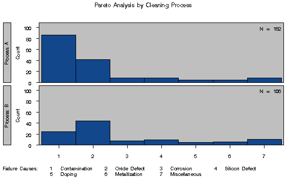
Output 29.2.2: One-Way Comparative Pareto Analysis with CLASS=PROCESS

Each cell corresponds to a level of the CLASS= variable (PROCESS). By default, the cells are arranged from top to bottom in alphabetical order of the formatted values of PROCESS, and the key cell is the top cell. The main difference in the two cells is a drop in contamination using Process B.

The CATLEGLABEL= option specifies the category legend label Failure Causes:. The NOHLABEL option suppresses the horizontal axis labels. The NOCURVE option suppresses the cumulative percent curve.

One-way Comparative Pareto Chart for DAY

The following statements specify DAY as a classification variable:

   title 'Pareto Analysis by Day';
   proc pareto data=failure4;
      vbar cause / class       = day
                   freq        = counts
                   last        = 'Miscellaneous'
                   scale       = count
                   cbars       = vigb
                   cframe      = ligr
                   cframetop   = ligr
                   catleglabel = 'Failure Causes:'
                   intertile   = 1.0
                   nrows       = 1
                   ncols       = 5
                   vref        = 5 10 15 20
                   lvref       = 34
                   nohlabel
                   nocurve
                   nlegend ;
   run;

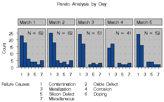
The NROWS= and NCOLS= options display the cells in a side-by-side arrangement. The VREF= and LVREF= options add reference lines. The chart is displayed in Output 29.2.3.

Output 29.2.3: One-Way Comparative Pareto Analysis with CLASS=DAY

By default, the key cell is the leftmost cell. There were no failures due to Metallization starting on March 3 (in fact, process controls to reduce this problem were introduced on this day).

Two-way Comparative Pareto Chart for PROCESS and DAY

The following statements specify both PROCESS and DAY as CLASS= variables to create a two-way comparative Pareto chart:

   title 'Pareto Analysis by Process and Day' ;
   proc pareto data=failure4;
      vbar cause / class       = ( process day )
                   freq        = counts
                   nrows       = 2
                   ncols       = 5
                   cbars       = vigb
                   cframe      = ligr
                   cframetop   = ligr
                   cframeside  = ligr
                   last        = 'Miscellaneous'
                   scale       = count
                   catleglabel = 'Failure Causes:'
                   intertile   = 1.0
                   nohlabel
                   nocurve
                   nlegend ;
   run;

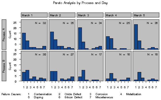
The chart is displayed in Output 29.2.4.

Output 29.2.4: Two-Way Comparative Pareto Analysis for PROCESS and DAY

The cells are arranged in a matrix whose rows correspond to levels of the first CLASS= variable (PROCESS) and whose columns correspond to levels of the second CLASS= variable (DAY). The dimensions of the matrix are specified with the NROWS= and NCOLS= options. The key cell is in the upper left corner. The chart reveals continuous improvement with Process B.

Chapter Contents
Previous
Next
Top