MANOVA Statement
- MANOVA < test-options >< / detail-options > ;
If the MODEL statement includes more than one
dependent variable, you can perform multivariate analysis of variance
with the MANOVA statement. The test-options define which effects
to test,
while the detail-options specify how to execute
the tests and what results to display.
When a MANOVA statement appears before the first RUN statement,
PROC GLM enters a multivariate mode with respect to the handling
of missing values; in addition to observations with missing independent
variables, observations with any missing dependent variables are
excluded from the analysis.
If you want to use this mode of handling missing
values and do not need any multivariate analyses,
specify the MANOVA option in the PROC GLM statement.
If you use both the CONTRAST and MANOVA statements, the
MANOVA statement must appear after the CONTRAST statement.
Test Options
The following options can be specified in the MANOVA statement
as test-options in order to define which multivariate tests
to perform.
- H=effects | INTERCEPT | _ALL_
-
specifies effects in the preceding
model to use as hypothesis matrices.
For each H matrix (the SSCP matrix associated with
an effect), the H= specification displays the characteristic
roots and vectors of E-1H (where E
is the matrix associated with the error effect),
Hotelling-Lawley trace, Pillai's trace, Wilks' criterion, and
Roy's maximum root criterion with approximate F statistic.
Use the keyword INTERCEPT to produce tests for the intercept.
To produce tests for all effects listed in the MODEL statement,
use the keyword _ALL_ in place of a list of effects.
For background and further details, see the "Multivariate Analysis of Variance" section.
- E=effect
-
specifies the error effect.
If you omit the E= specification, the GLM procedure uses the
error SSCP (residual) matrix from the analysis.
- M=equation,...,equation |
(row-of-matrix,...,row-of-matrix)
-
specifies a transformation matrix for the
dependent variables listed in the MODEL statement.
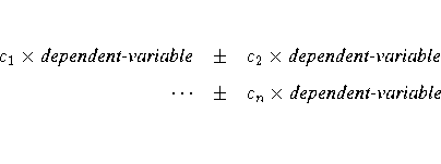
The equations in the M= specification are of the form

where the ci values are coefficients
for the various dependent-variables.
If the value of a given ci is 1, it can be omitted;
in other words 1 ×Y is the same as Y.
Equations should involve two or more dependent variables.
For sample syntax, see the "Examples" section.
Alternatively, you can input the transformation matrix
directly by entering the elements of the matrix with commas
separating the rows and parentheses surrounding the matrix.
When this alternate form of input is used, the number of elements
in each row must equal the number of dependent variables.
Although these combinations actually represent the
columns of the M matrix, they are displayed by rows.
When you include an M= specification, the analysis
requested in the MANOVA statement is carried out
for the variables defined by the equations in the
specification, not the original dependent variables.
If you omit the M= option, the analysis is performed for the
original dependent variables in the MODEL statement.
If an M= specification is included without either
the MNAMES= or PREFIX= option, the variables are
labeled MVAR1, MVAR2, and so forth, by default.
For further information, see the "Multivariate Analysis of Variance" section.
- MNAMES=names
-
provides names for the variables defined
by the equations in the M= specification.
Names in the list correspond to the M= equations or to
the rows of the M matrix (as it is entered).
- PREFIX=name
-
is an alternative means of identifying the
transformed variables defined by the M= specification.
For example, if you specify PREFIX=DIFF, the transformed
variables are labeled DIFF1, DIFF2, and so forth.
Detail Options
You can specify the following options in
the MANOVA statement after a slash as detail-options.
- CANONICAL
-
displays a canonical analysis of the H and
E matrices (transformed by the M
matrix, if specified) instead of the default
display of characteristic roots and vectors.
- ETYPE=n
-
specifies the type (1, 2, 3, or 4, corresponding to Type I, II, III, and
IV tests, respectively) of the E matrix, the SSCP matrix associated
with the E= effect.
You need this option if you use the E= specification
to specify an error effect other than residual error and you want to
specify the type of sums of squares used for the effect.
If you specify ETYPE=n, the corresponding test must have been
performed in the MODEL statement, either by options
SSn, En, or the default Type I and Type III tests.
By default, the procedure uses an ETYPE= value corresponding
to the highest type (largest n) used in the analysis.
- HTYPE=n
-
specifies the type (1, 2, 3, or 4, corresponding to Type I, II, III, and
IV tests, respectively) of the H matrix.
See the ETYPE= option for more details.
- ORTH
-
requests that the transformation matrix in the
M= specification of the MANOVA statement be
orthonormalized by rows before the analysis.
- PRINTE
-
displays the error SSCP matrix E.
If the E matrix is the error SSCP (residual) matrix
from the analysis, the partial correlations of the dependent
variables given the independent variables are also produced.
For example, the statement
manova / printe;
displays the error SSCP matrix and the partial
correlation matrix computed from the error SSCP matrix.
- PRINTH
-
displays the hypothesis SSCP matrix H associated
with each effect specified by the H= specification.
- SUMMARY
-
produces analysis-of-variance
tables for each dependent variable.
When no M matrix is specified, a table is displayed for
each original dependent variable from the MODEL statement; with
an M matrix other than the identity, a table is displayed
for each transformed variable defined by the M matrix.
The following statements provide several
examples of using a MANOVA statement.
   proc glm;
      class A B;
      model Y1-Y5=A B(A) / nouni;
      manova h=A e=B(A) / printh printe htype=1 etype=1;
      manova h=B(A) / printe;
      manova h=A e=B(A) m=Y1-Y2,Y2-Y3,Y3-Y4,Y4-Y5
             prefix=diff;
      manova h=A e=B(A) m=(1 -1  0  0  0,
                           0  1 -1  0  0,
                           0  0  1 -1  0,
                           0  0  0  1 -1) prefix=diff;
   run;
Since this MODEL statement requests no options for
type of sums of squares, the procedure uses Type I
and Type III sums of squares.
The first MANOVA statement specifies A as the
hypothesis effect and B(A) as the error effect.
As a result of the PRINTH option, the procedure displays the
hypothesis SSCP matrix associated with the A effect; and,
as a result of the PRINTE option, the procedure displays the
error SSCP matrix associated with the B(A) effect.
The option HTYPE=1 specifies a Type I H matrix, and
the option ETYPE=1 specifies a Type I E matrix.
The second MANOVA statement specifies
B(A) as the hypothesis effect.
Since no error effect is specified, PROC GLM uses the error
SSCP matrix from the analysis as the E matrix.
The PRINTE option displays this E matrix.
Since the E matrix is the error SSCP
matrix from the analysis, the partial correlation
matrix computed from this matrix is also produced.
The third MANOVA statement requests the same analysis
as the first MANOVA statement, but the analysis is
carried out for variables transformed to be successive
differences between the original dependent variables.
The option PREFIX=DIFF labels the transformed
variables as DIFF1, DIFF2, DIFF3, and DIFF4.
Finally, the fourth MANOVA statement has the
identical effect as the third, but it uses
an alternative form of the M= specification.
Instead of specifying a set of equations, the
fourth MANOVA statement specifies rows of a matrix
of coefficients for the five dependent variables.
As a second example of the use of the M=
specification, consider the following:
   proc glm;
      class group;
      model dose1-dose4=group / nouni;
      manova h = group
             m = -3*dose1 -   dose2 +   dose3 + 3*dose4,
                    dose1 -   dose2 -   dose3 +   dose4,
                   -dose1 + 3*dose2 - 3*dose3 +   dose4
             mnames = Linear Quadratic Cubic
             / printe;
   run;
The M= specification gives a transformation of the dependent
variables dose1 through dose4 into orthogonal polynomial
components, and the MNAMES= option labels the transformed
variables LINEAR, QUADRATIC, and CUBIC, respectively.
Since the PRINTE option is specified and the default residual
matrix is used as an error term, the partial correlation
matrix of the orthogonal polynomial components is also produced.
Copyright © 1999 by SAS Institute Inc., Cary, NC, USA. All rights reserved.
