Chapter Contents
Previous
Next
|
Chapter Contents |
Previous |
Next |
| The KRIGE2D Procedure |
As an illustration, consider a hypothetical example in which
an organic solvent leaks from an industrial site
and spreads over a large area. Assume the solvent
is absorbed and immobilized into the subsoil
above any ground-water level, so you can ignore any time dependence.
For you to find the areal extent
and the concentration values
of the solvent, measurements are required.
Although the problem is inherently three-dimensional,
if you measure total concentration in a column of soil
or take a depth-averaged concentration, it can be
handled reasonably well with two-dimensional techniques.
You usually assume that measured
concentrations are higher closer to the
source and decrease at larger
distances from the source. On top of this
smooth variation, there are small-scale
variations in the measured concentrations, due
perhaps to the inherent variability of soil properties.
You also tend to suspect that measurements
made close together yield similar
concentration values, while measurements
made far apart can have very different values.
These physically reasonable qualitative statements
have no explicit probabilistic content, and there are a number
of numerical smoothing techniques, such as inverse
distance weighting and splines, that make use of large-scale
variations and
"close distance-close value"
characteristics of spatial data to interpolate the measured
concentrations for contouring purposes.
While characteristics (i) and (iii) are handled by
such smoothing methods, characteristic (ii), the small-scale
residual variation in the concentration field,
is not accounted for.
There may be situations, due to the use of the
prediction map or
due to the relative magnitude of the irregular
fluctuations, where you cannot ignore these small-scale
irregular fluctuations. In other words, the smoothed or
estimated values of the concentration field alone are
not a sufficient characterization; you also need the possible spread
around these contoured values.
The key assumption in applying the SRF formalism is that
the measurements come from a single realization of the
SRF. However, in most geostatistical applications, the
focus is on a single, unique realization. This is
unlike most other situations in stochastic
modeling in which there will be future experiments
or observational activities (at least conceptually)
under similar circumstances. This renders many
traditional ideas of statistical
inference ambiguous and somewhat
counterintuitive.
There are additional logical and methodological
problems in applying a stochastic model to a unique
but partly unknown natural process; refer to the
introduction in
Matheron (1971) and
Cressie (1993, section 2.3).
These difficulties have resulted in
attempts to frame the estimation problem in a
completely deterministic way
(Isaaks and Srivastava 1988;
Journel 1985).
Additional problems with kriging, and with spatial
estimation methods in general, are related to the
necessary assumption of ergodicity of the spatial process.
This assumption is required to estimate the
covariance or semivariogram from sample data.
Details are provided in Cressie (1993, pp. 52 -58).
Despite these difficulties, ordinary kriging remains a popular and
widely used tool in modeling spatial data, especially
in generating surface plots and contour maps.
An abbreviated derivation
of the OK estimator for point estimation and the
associated standard error is discussed in the following
section.
Full details are given in
Journel and Huijbregts (1978), Christakos (1992),
and Cressie (1993).
Here,
In most practical applications, an additional assumption is
required in order to estimate the covariance Cz of
the Z(r) process. This assumption is
second-order stationarity:
This requirement can be relaxed slightly
when you are using the semivariogram
instead of the covariance. In this case,
second-order
stationarity is required of the differences
By performing local kriging, the spatial processes
represented by the previous equation for Z(r) are more general than
they appear. In local kriging, at an unsampled location
r0, a separate model is fit using only data
in a neighborhood of r0. This has the effect of
fitting a separate mean
Given the N measurements Z(r1), ... , Z(rN) at
known locations r1, ... ,rN,
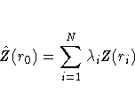
you want to obtain an estimate Linearity requires the following form for
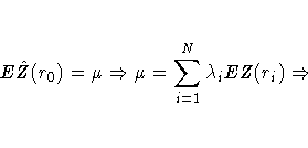
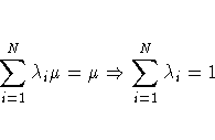
Applying the unbiasedness condition to the preceding equation yields
Finally, the third condition requires a constrained
linear optimization involving
Define the N ×1 column vector The optimization is performed by solving
The resulting matrix equation can be expressed in
terms of either the covariance Cz(r) or
semivariogram
The solution to the previous matrix equation is
Using this solution for
with associated prediction error
where c0 is C0 with the 1 in the last row removed, making
it an N ×1 vector.
These formulas are used in the
best linear unbiased prediction (BLUP)
of random variables (Robinson
1991). Further details are provided in
Cressie (1993, pp. 119 -123).
Because of possible numeric problems when solving
the previous matrix equation,
Duetsch and Journel (1992)
suggest replacing the last
row and column of 1s in the preceding matrix
C by
Cz(0), keeping the 0 in the (N+1,N+1) position
and similarly replacing the last element in the
preceding right-hand vector C0
with Cz(0). This results in an
equivalent system but avoids numeric problems when
Cz(0) is large or small relative to 1.
Copyright © 1999 by SAS Institute Inc., Cary, NC, USA. All rights reserved.
Spatial Random Fields
One method of incorporating characteristic (ii) into the
construction of a contour map is to model the concentration
field as a spatial random field (SRF). The mathematical
details of SRF models are given in a number of texts,
for example, Cressie (1993) and Christakos (1992). The mathematics
of SRFs are formidable. However, under certain simplifying
assumptions, they produce classical linear estimators with
very simple properties, allowing easy
implementation for prediction purposes. These estimators,
primarily ordinary kriging (OK), give both a prediction
and a standard error of prediction at unsampled locations.
This allows the construction of a map of both predicted
values and level of uncertainty about the predicted
values.
Ordinary Kriging
Denote the SRF by ![]() .Following the notation in
Cressie (1993), the following model
for Z(r) is assumed:
.Following the notation in
Cressie (1993), the following model
for Z(r) is assumed:

![]() is the fixed, unknown mean of the process,
and
is the fixed, unknown mean of the process,
and ![]() is a zero mean SRF representing
the variation around the mean.
is a zero mean SRF representing
the variation around the mean.
![C_z(r_1,r_2)
= E[\varepsilon(r_1)\varepsilon(r_2)]
= C_z(r_1-r_2)](images/krieq49.gif)
![]() rather than
rather than ![]() :
:![\gamma_Z(r_1,r_2) =
\frac{1}2E[\varepsilon(r_1)-\varepsilon(r_2)]^2
= \gamma_Z(r_1-r_2)](images/krieq51.gif)
![]() at each point, and it
is similar to
the "kriging with trend" (KT)
method discussed in Journel and Rossi (1989).
at each point, and it
is similar to
the "kriging with trend" (KT)
method discussed in Journel and Rossi (1989).
![]() of Z at an
unsampled location r0.
When the following three requirements are
imposed on the estimator
of Z at an
unsampled location r0.
When the following three requirements are
imposed on the estimator ![]() ,the OK estimator is obtained.
,the OK estimator is obtained.
![]() is linear
in Z(r1), ... , Z(rN).
is linear
in Z(r1), ... , Z(rN).
![]() is unbiased.
is unbiased.
![]() minimizes the mean-square prediction
error
minimizes the mean-square prediction
error ![]() .
.
![]() :
:
![]() and
a Lagrange parameter 2m. This constrained
linear optimization can be expressed in terms of the
function
and
a Lagrange parameter 2m. This constrained
linear optimization can be expressed in terms of the
function ![]() given by
given by

![]() by
by
and the (N+1) ×1 column vector 
![]() by
by
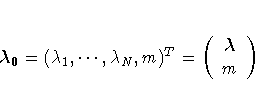
in terms of 
![]() and m.
and m.
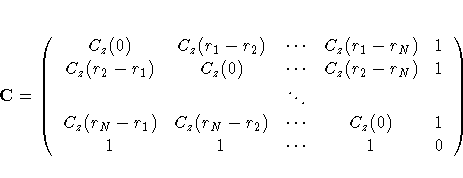
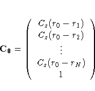
![]() .In terms of the covariance, the preceding equation results
in the following
matrix equation:
.In terms of the covariance, the preceding equation results
in the following
matrix equation:
where

and

![]() and m, the
ordinary kriging estimate at r0 is
and m, the
ordinary kriging estimate at r0 is


![]()
Chapter Contents
![]()
Previous
![]()
Next
![]()
Top