Chapter Contents
Previous
Next
|
Chapter Contents |
Previous |
Next |
| The KRIGE2D Procedure |
In all the theoretical models considered previously,
the lag distance h entered as a scalar value.
This implies that the correlation between the spatial
process at two point pairs
P1,P2 is dependent only on the separation
distance h = | P1P2 |, not on the orientation
of the two points.
A spatial process {![]() }
with this property is called isotropic, as is
the associated covariance or semivariogram.
}
with this property is called isotropic, as is
the associated covariance or semivariogram.
However, real spatial phenomena often show directional effects. Particularly in geologic applications, measurements along a particular direction may be highly correlated, while the perpendicular direction shows little or no correlation. Such processes are called anisotropic. Refer to Journel and Huijbregts (1978, section III.B.4) for more details.
There are two types of anisotropy. The simplest type occurs when the same covariance form and scale parameter c0 is present in all directions but the range a0 changes with direction. In this case, there is a single sill, but the semivariogram reaches the sill in a shorter lag distance along a certain direction.
This type of anisotropy is called "geometric" and is discussed in the following section.

|
As you can see from the figure, the SE -NW curve gets "close" to the sill at approximately h=2, while the NE -SW curve does so at h=6. The ratio of the shorter to longer distance is (2/6) = (1/3). This is the value to use in the RATIO= parameter in the MODEL statement in PROC KRIGE2D. Since the longer, or major, axis is in the NE -SW direction, the ANGLE= parameter in the MODEL statement in PROC KRIGE2D should be 45o (all angles are measured clockwise from north).
The terminology associated with geometric anisotropy is that of ellipses. To see how this comes about, consider the following hypothetical set of calculations.
Let {![]() } be a
geometrically anisotropic process,
and assume that there are sufficient
data points to calculate an experimental semivariogram
at a large number of angle classes
} be a
geometrically anisotropic process,
and assume that there are sufficient
data points to calculate an experimental semivariogram
at a large number of angle classes ![]() }. At each of these
angles
}. At each of these
angles ![]() , the experimental semivariogram is plotted
and the effective range
, the experimental semivariogram is plotted
and the effective range ![]() is recorded.
A diagram, in polar coordinates, of
is recorded.
A diagram, in polar coordinates, of ![]() yields an ellipse, with the major axis in the direction of
the largest
yields an ellipse, with the major axis in the direction of
the largest ![]() and the minor axis perpendicular.
Denote the largest
and the minor axis perpendicular.
Denote the largest ![]() by
by
![]() , the smallest by
, the smallest by
![]() , and their ratio by
, and their ratio by

By a rotation, a new set of axes are aligned along the major and minor axis. Then, a rescaling elongates the minor axis so its length equals that of the major axis of the ellipse.
First, the angle ![]() of
the major axis of the ellipse (measured clockwise from north)
is transformed to standard
Cartesian orientation or counter-clockwise from the x-axis
(east). Let
of
the major axis of the ellipse (measured clockwise from north)
is transformed to standard
Cartesian orientation or counter-clockwise from the x-axis
(east). Let ![]() denote the transformed angle.
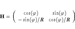
The matrix to transform the distance h is in terms of
denote the transformed angle.
The matrix to transform the distance h is in terms of
![]() and the ratio R and it is given by
and the ratio R and it is given by

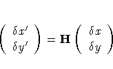
For a given point pair P1P2, with coordinates
(x1,y1), (x2,y2), the transformed interpair
distance is computed by first transforming the
components ![]() and
and
![]() by
by

The transformed interpair distance is then

The original semivariogram, a function of both
h and ![]() , is then transformed to a function
only of h':
, is then transformed to a function
only of h':

This single semivariogram is then used for kriging purposes.
The interpretation of the major/minor axis in the case of
geometric anisotropy is that
the direction of the major axis is the direction in which
the spatial process ![]() is most highly
correlated; the process is least correlated in the
perpendicular direction.
is most highly
correlated; the process is least correlated in the
perpendicular direction.
In some cases, these directions are known a priori. This can occur in mining applications where the geology of a region is known in advance. In most cases, however, nothing is known about possible anisotropy. Depending on the amount of data available, using four to six directions is usually sufficient to determine the presence of anisotropy and find the approximate major/minor axis directions.
The most convenient way of performing this is to
use the NDIR= option in the COMPUTE statement in
PROC VARIOGRAM to obtain
a separate experimental semivariogram for
each direction. After determining the direction of the
major axis, use a DIRECTIONS statement on a subsequent
run of PROC VARIOGRAM with this direction and its
perpendicular direction. For example, if the
initial run of PROC VARIOGRAM with NDIR=6 in the
COMPUTE statement indicates that ![]() is the major axis (has the largest
is the major axis (has the largest ![]() ),
then rerun PROC VARIOGRAM with
),
then rerun PROC VARIOGRAM with
DIRECTIONS 45,135;
Then, determine the ratio of ![]() for
the minor and major axis for the RATIO= parameter
in the COMPUTE statement of
PROC KRIGE2D. This ratio is
for
the minor and major axis for the RATIO= parameter
in the COMPUTE statement of
PROC KRIGE2D. This ratio is ![]() for
modeling geometric anisotropy.
In the other type of anisotropy,
zonal anisotropy, the
RATIO= parameter is set to a large number
for reasons explained in the following section.
for
modeling geometric anisotropy.
In the other type of anisotropy,
zonal anisotropy, the
RATIO= parameter is set to a large number
for reasons explained in the following section.
Instead, nesting and geometric anisotropy are used together
to approximate zonal anisotropy. For example,
suppose the spatial process has a correlation structure in
the N -S direction described by ![]() , a spherical model with
sill at c0=6 and range a0=2, while in the
E -W direction the correlation structure,
described by
, a spherical model with
sill at c0=6 and range a0=2, while in the
E -W direction the correlation structure,
described by ![]() , is again a spherical
model but with
sill at c0=3 and range a0=1.
, is again a spherical
model but with
sill at c0=3 and range a0=1.
You can approximate this structure in PROC KRIGE2D by specifying two nested models with large RATIO= values. In particular, the appropriate MODEL statement is
   MODEL FORM=(S,S) ANGLE=(0,90) SCALE=(6,3)
         RANGE=(2,1) RATIO=(1E8,1E8);
The large values of the RATIO= parameter for
each nested structure
have the effect of an "infinite" range parameter
in the direction of the minor axis. Hence, there
is no variation in ![]() in the E -W direction
and no variation in
in the E -W direction
and no variation in ![]() in the N -S direction.
in the N -S direction.
|
Chapter Contents |
Previous |
Next |
Top |
Copyright © 1999 by SAS Institute Inc., Cary, NC, USA. All rights reserved.