PROC MDS Statement

The MDS Procedure

PROC MDS Statement

PROC MDS < options > ;

By default, the only result produced by the MDS procedure is the iteration history. Hence, you should always specify one or more options for output data sets (OUT=, OUTFIT=, and OUTRES=) or displayed output (such as PFINAL). PROC MDS does not produce any plots; to produce plots, use the output data sets with PROC PLOT or PROC GPLOT.

The types of estimates written to the OUT= data set are determined by the OCONFIG, OCOEF, OTRANS, and OCRIT options. If you do not specify any of these four options, the estimates of all the parameters of the PROC MDS model and the value of the badness-of-fit criterion appear in the OUT= data set. If you specify one or more of these options, only the information requested by the specified options appear in the OUT= data set. Also, the OITER option causes these statistics to be written to the OUT= data set after initialization and on each iteration, as well as after the iterations have terminated.

Displayed output is controlled by the interaction of the PCONFIG, PCOEF, PTRANS, PFIT, and PFITROW options with the PININ, PINIT, PITER, and PFINAL options. The PCONFIG, PCOEF, PTRANS, PFIT, and PFITROW options specify which estimates and fit statistics are to be displayed. The PININ, PINIT, PITER, and PFINAL options specify when the estimates and fit statistics are to be displayed. If you specify at least one of the PCONFIG, PCOEF, PTRANS, PFIT and PFITROW options but none of the PININ, PINIT, PITER, and PFINAL options, the final results (PFINAL) are displayed. If you specify at least one of the PININ, PINIT, PITER, and PFINAL options but none of the PCONFIG, PCOEF, PTRANS, PFIT and PFITROW options, all estimates (PCONFIG, PCOEF, PTRANS) and the fit statistics for each matrix and for the entire sample (PFIT) are displayed. If you do not specify any of these nine options, no estimates or fit statistics are displayed (except the badness-of-fit criterion in the iteration history).

ALTERNATE | ALT=NONE | NO | N

ALTERNATE | ALT=MATRIX | MAT | M | SUBJECT | SUB | S

ALTERNATE | ALT=ROW | R <=n>

determines what form of alternating-least-squares algorithm is used. The default depends on the amount of memory available. The following ALTERNATE= options are listed in order of decreasing memory requirements:

ALT=NONE: causes all parameters to be adjusted simultaneously on each iteration. This option is usually best for a small number of subjects and objects.
ALT=MATRIX: adjusts all the parameters for the first subject, then all the parameters for the second subject, and so on, and finally adjusts all parameters that do not correspond to a subject, such as coordinates and unconditional transformations. This option usually works best for a large number of subjects with a small number of objects.
ALT=ROW: treats subject parameters the same way as the ALTERNATE=MATRIX option but also includes separate stages for unconditional parameters and for subsets of the objects. The ALT=ROW option usually works best for a large number of objects.

Specifying ALT=ROW=n divides the objects into subsets of n objects each, except possibly for one subset when n does not divide the number of objects evenly. If you omit =n, the number of objects in the subsets is determined from the amount of memory available. The smaller the value of n, the less memory is required.

When you specify the LEVEL=ORDINAL option, the monotone transformation is always computed in a separate stage and is listed as a separate iteration in the iteration history. In this case, estimation is done by iteratively reweighted least squares. The weights are recomputed according to the FORMULA= option on each monotone iteration; hence, it is possible for the badness-of-fit criterion to increase after a monotone iteration.

COEF=IDENTITY | IDEN | I

COEF=DIAGONAL | DIAG | D

specifies the type of matrix for the dimension coefficients.

COEF=IDENTITY: is the default, which yields Euclidean distances.
COEF=DIAGONAL: produces weighted Euclidean distances, in which each subject is allowed differential weights for the dimensions. The dimension coefficients that PROC MDS outputs are related to the square roots of what are called subject weights in PROC ALSCAL; the normalization in PROC MDS also differs from that in PROC ALSCAL. The weighted Euclidean model is related to the INDSCAL model (Carroll and Chang 1970).

CONDITION | COND=UN | U

CONDITION | COND=MATRIX | MAT | M | SUBJECT | SUB | S

CONDITION | COND=ROW | R

specifies the conditionality of the data (Young 1987, pp. 60-63). The default is CONDITION=MATRIX.

The data are divided into disjoint subsets called partitions. Within each partition, a separate transformation is applied, as specified by the LEVEL= option.

COND=UN: puts all the data into a single partition.
COND=MATRIX: makes each data matrix a partition.
COND=ROW: makes each row of each data matrix a partition.

The CONDITION= option also determines the default value for the SHAPE= option. If you specify the CONDITION=ROW option and omit the SHAPE= option, each data matrix is stored as a square and possibly asymmetric matrix. If you specify the CONDITION=UN or CONDITION=MATRIX option and omit the SHAPE= option, only one triangle is stored. See the SHAPE= option for details.

CONVERGE | CONV=p

sets both the gradient convergence criterion and the monotone convergence criterion to p, where $0 \leq p \leq 1$ . The default is CONVERGE=.01; smaller values may greatly increase the number of iterations required. Values less than .0001 may be impossible to satisfy because of the limits of machine precision. See the GCONVERGE= and MCONVERGE= options.

CUTOFF=n

causes data less than n to be replaced by missing values. The default is CUTOFF=0.

DATA=SAS-data-set

specifies the SAS data set containing one or more square matrices to be analyzed. In typical psychometric data, each matrix contains judgments from one subject, so there is a one-to-one correspondence between data matrices and subjects.

The data matrices contain similarity or dissimilarity measurements to be modeled and, optionally, weights for these data. The data are generally assumed to be dissimilarities unless you use the SIMILAR option. However, if there are nonmissing diagonal values and these values are predominantly larger than the off-diagonal values, the data are assumed to be similarities and are treated as if the SIMILAR option is specified. The diagonal elements are not otherwise used in fitting the model.

Each matrix must have exactly the same number of observations as the number of variables specified by the VAR statement or determined by defaults. This number is the number of objects or stimuli.

The first observation and variable are assumed to contain data for the first object, the second observation and variable are assumed to contain data for the second object, and so on.

When there are two or more matrices, the observations in each matrix must correspond to the same objects in the same order as in the first matrix.

The matrices can be symmetric or asymmetric, as specified by the SHAPE= option.

DECIMALS | DEC=n

specifies how many decimal places to use when displaying the parameter estimates and fit statistics. The default is DECIMALS=2, which is generally reasonable except in conjunction with the LEVEL=ABSOLUTE option and very large or very small data.

DIMENSION | DIMENS | DIM=n < TO m < BY=i >>

specifies the number of dimensions to use in the MDS model, where $1 \leq n, m \lt$ number of objects. The parameter i can be either positive or negative but not zero. If you specify different values for n and m, a separate model is fitted for each requested dimension. If you specify only DIMENSION=n, then only n dimensions are fitted. The default is DIMENSION=2 if there are three or more objects; otherwise, DIMENSION=1 is the only valid specification. The analyses for each number of dimensions are done independently. For information on choosing the dimensionality, refer to Kruskal and Wish (1978, pp. 48-60).

EPSILON | EPS=n

specifies a number n, 0 < n < 1, that determines the amount added to squared distances computed from the model to avoid numerical problems such as division by 0. This amount is computed as ${\epsilon}$ equal to n times the mean squared distance in the initial configuration. The distance in the MDS model is thus computed as

$distance = {\sqrt{sqdist + \epsilon}}$

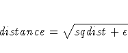
where sqdist is the squared Euclidean distance or the weighted squared Euclidean distance.

The default is EPSILON=1E-12, which is small enough to have no practical effect on the estimates unless the FIT= value is nonpositive and there are dissimilarities that are very close to 0. Hence, when the FIT= value is nonpositive, dissimilarities less than n times 100 times the maximum dissimilarity are disallowed.

FIT=DISTANCE | DIS | D

FIT=SQUARED | SQU | S

FIT=LOG | L

FIT=n

specifies a predetermined (not estimated) transformation to apply to both sides of the MDS model before the error term is added.

The default is FIT=DISTANCE or, equivalently, FIT=1, which fits data to distances.

The option FIT=SQUARED or FIT=2 fits squared data to squared distances. This gives greater importance to large data and distances and lesser importance to small data and distances in fitting the model.

The FIT=LOG or FIT=0 option fits log data to log distances. This gives lesser importance to large data and distances and greater importance to small data and distances in fitting the model.

In general, the FIT=n option fits nth-power data to nth-power distances. Values of n that are large in absolute value can cause floating-point overflows.

If the FIT= value is 0 or negative, the data must be strictly positive (see the EPSILON= option). Negative data may produce strange results with any value other than FIT=1.

FORMULA | FOR=0 | OLS | O

FORMULA | FOR=1 | USS | U

FORMULA | FOR=2 | CSS | C

determines how the badness-of-fit criterion is standardized in correspondence with stress formulas 1 and 2 (Kruskal and Wish 1978, pp. 24-26). The default is FORMULA=1 unless you specify FIT=LOG, in which case the default is FORMULA=2. Data partitions are defined by the CONDITION= option.

FORMULA=0: fits a regression model by ordinary least squares (Null and Sarle 1982) without standardizing the partitions; this option cannot be used with the LEVEL=ORDINAL option. The badness-of-fit criterion is the square root of the error sum of squares.
FORMULA=1: standardizes each partition by the uncorrected sum of squares of the (possibly transformed) data; this option should not be used with the FIT=LOG option. With the FIT=DISTANCE and LEVEL=ORDINAL options, this is equivalent to Kruskal's stress formula 1 or an obvious generalization thereof. With the FIT=SQUARED and LEVEL=ORDINAL options, this is equivalent to Young's s-stress formula 1 or an obvious generalization thereof. The badness-of-fit criterion is analogous to $\sqrt{1-R^2}$ , where R is a multiple correlation about the origin.
FORMULA=2: standardizes each partition by the corrected sum of squares of the (possibly transformed) data; this option is the recommended method for unfolding. With the FIT=DISTANCE and LEVEL=ORDINAL options, this is equivalent to Kruskal's stress formula 2 or an obvious generalization thereof. With the FIT=SQUARED and LEVEL=ORDINAL options, this is equivalent to Young's s-stress formula 2 or an obvious generalization thereof. The badness-of-fit criterion is analogous to $\sqrt{1-R^2}$ , where R is a multiple correlation computed with a denominator corrected for the mean.

GCONVERGE | GCONV=p

sets the gradient convergence criterion to p, where $0 \leq p \leq 1$ . The default is GCONVERGE=0.01; smaller values may greatly increase the number of iterations required. Values less than 0.0001 may be impossible to satisfy because of the limits of machine precision.

The gradient convergence measure is the multiple correlation of the Jacobian matrix with the residual vector, uncorrected for the mean. See the CONVERGE= and MCONVERGE= options.

INAV=DATA | D

INAV=SSCP | S

affects the computation of initial coordinates. The default is INAV=DATA.

INAV=DATA: computes a weighted average of the data matrices. Its value is estimated only if an element is missing from every data matrix. The weighted average of the data matrices with missing values filled in is then converted to a scalar products matrix (or what would be a scalar products matrix if the fit were perfect), from which the initial coordinates are computed.
INAV=SSCP: estimates missing values in each data matrix and converts each data matrix to a scalar products matrix. The initial coordinates are computed from the unweighted average of the scalar products matrices.

INITIAL | IN=SAS-data-set

specifies a SAS data set containing initial values for some or all of the parameters of the MDS model. If the INITIAL= option is omitted, the initial values are computed from the data.

LEVEL=ABSOLUTE | ABS | A

LEVEL=RATIO | RAT | R

LEVEL=INTERVAL | INT | I

LEVEL=LOGINTERVAL | LOG | L

LEVEL=ORDINAL | ORD | O

specifies the measurement level of the data and hence the type of estimated (optimal) transformations applied to the data or distances (Young 1987, pp. 57-60; Krantz et. al. 1971, pp. 9-12) within each partition as specified by the CONDITION= option. The default is LEVEL=ORDINAL.

LEVEL=ABSOLUTE: allows no optimal transformations. Hence, the distinction between regression and measurement models is irrelevant.
LEVEL=RATIO: fits a regression model in which the distances are multiplied by a slope parameter in each partition (a linear transformation). In this case, the regression model is equivalent to the measurement model with the slope parameter reciprocated.
LEVEL=INTERVAL: fits a regression model in which the distances are multiplied by a slope parameter and added to an intercept parameter in each partition (an affine transformation). In this case, the regression and measurement models differ if there is more than one partition.
LEVEL=LOGINTERVAL: fits a regression model in which the distances are raised to a power and multiplied by a slope parameter in each partition (a power transformation).
LEVEL=ORDINAL: fits a measurement model in which a least-squares monotone increasing transformation is applied to the data in each partition. At the ordinal measurement level, the regression and measurement models differ.

MAXITER | ITER=n

specifies the maximum number of iterations, where $n \geq 0$ . The default is MAXITER=100.

MCONVERGE | MCONV=p

sets the monotone convergence criterion to p, where $0 \leq p \leq 1$ , for use with the LEVEL=ORDINAL option. The default is MCONVERGE=0.01; if you want greater precision, MCONVERGE=0.001 is usually reasonable, but smaller values may greatly increase the number of iterations required.

The monotone convergence criterion is the Euclidean norm of the change in the optimally scaled data divided by the Euclidean norm of the optimally scaled data, averaged across partitions defined by the CONDITION= option. See the CONVERGE= and GCONVERGE= options.

MINCRIT | CRITMIN=n

causes iteration to terminate when the badness-of-fit criterion is less than or equal to n, where $n \geq 0$ . The default is MINCRIT=1E-6.

NEGATIVE

allows slopes or powers to be negative with the LEVEL=RATIO, INTERVAL, or LOGINTERVAL option.

NONORM

suppresses normalization of the initial and final estimates.

NOPHIST | NOPRINT | NOP

suppresses the output of the iteration history.

NOULB

causes missing data to be estimated during initialization by the average nonmissing value, where the average is computed according to the FIT= option. Otherwise, missing data are estimated by interpolating between the Rabinowitz (1976) upper and lower bounds.

OCOEF

writes the dimension coefficients to the OUT= data set. See the OUT= option for interactions with other options.

OCONFIG

writes the coordinates of the objects to the OUT= data set. See the OUT= option for interactions with other options.

OCRIT

writes the badness-of-fit criterion to the OUT= data set. See the OUT= option for interactions with other options.

OITER | OUTITER

writes current values to the output data sets after initialization and on every iteration. Otherwise, only the final values are written to any output data sets. See the OUT=, OUTFIT=, and OUTRES= options.

OTRANS

writes the transformation parameter estimates to the OUT= data set if any such estimates are computed. There are no transformation parameters with the LEVEL=ORDINAL option. See the OUT= option for interactions with other options.

OUT=SAS-data-set

creates a SAS data set containing, by default, the estimates of all the parameters of the PROC MDS model and the value of the badness-of-fit criterion. However, if you specify one or more of the OCONFIG, OCOEF, OTRANS, and OCRIT options, only the information requested by the specified options appears in the OUT= data set. See also the OITER option.

OUTFIT=SAS-data-set

creates a SAS data set containing goodness-of-fit and badness-of-fit measures for each partition as well as for the entire data set. See also the OITER option.

OUTRES=SAS-data-set

creates a SAS data set containing one observation for each nonmissing datum from the DATA= data set. Each observation contains the original datum, the estimated distance computed from the MDS model, transformed data and distances, and the residual. See also the OITER option.

OVER=n

specifies the maximum overrelaxation factor, where $n \geq 1$ . Values between 1 and 2 are generally reasonable. The default is OVER=2 with the LEVEL=ORDINAL, ALTERNATE=MATRIX, or ALTERNATE=ROW option; otherwise, the default is OVER=1. Use this option only if you have convergence problems.

PCOEF

produces the estimated dimension coefficients.

PCONFIG

produces the estimated coordinates of the objects in the configuration.

PDATA

displays each data matrix.

PFINAL

displays final estimates.

PFIT

displays the badness-of-fit criterion and various types of correlations between the data and fitted values for each data matrix, as well as for the entire sample.

PFITROW

displays the badness-of-fit criterion and various types of correlations between the data and fitted values for each row as well as for each data matrix and for the entire sample. This option works only with the CONDITION=ROW option.

PINAVDATA

displays the sum of the weights and the weighted average of the data matrices computed during initialization with the INAV=DATA option.

PINEIGVAL

displays the eigenvalues computed during initialization.

PINEIGVEC

displays the eigenvectors computed during initialization.

PININ

displays values read from the INITIAL= data set. Since these values may be incomplete, the PFIT and PFITROW options do not apply.

PINIT

displays initial values.

PITER

displays estimates on each iteration.

PTRANS

displays the estimated transformation parameters if any are computed. There are no transformation parameters with the LEVEL=ORDINAL option.

RANDOM<=seed>

causes initial coordinate values to be pseudorandom numbers. In one dimension, the pseudorandom numbers are uniformly distributed on an interval. In two or more dimensions, the pseudorandom numbers are uniformly distributed on the circumference of a circle or the surface of a (hyper)sphere.

RIDGE=n

specifies the initial ridge value, where $n \geq 0$ . The default is RIDGE=1E-4.

If you get a floating-point overflow in the first few iterations, specify a larger value such as RIDGE=0.01 or RIDGE=1 or RIDGE=100.

If you know that the initial estimates are very good, using RIDGE=0 may speed convergence.

SHAPE=TRIANGULAR | TRIANGLE | TRI | T

SHAPE=SQUARE | SQU | S

determines whether the entire data matrix for each subject or only one triangle of the matrix is stored and analyzed. If you specify the CONDITION=ROW option, the default is SHAPE=SQUARE. Otherwise, the default is SHAPE=TRIANGLE.

SHAPE=SQUARE: causes the entire matrix to be stored and analyzed. The matrix can be asymmetric.
SHAPE=TRIANGLE: causes only one triangle to be stored. However, PROC MDS reads both upper and lower triangles to look for nonmissing values and to symmetrize the data if needed. If corresponding elements in the upper and lower triangles both contain nonmissing values, only the average of the two values is stored and analyzed (Kruskal and Wish 1978, p. 74). Also, if an OUTRES= data set is requested, only the average of the two corresponding elements is output.

SIMILAR | SIM<=max>

causes the data to be treated as similarity measurements rather than dissimilarities. If =max is not specified, each datum is converted to a dissimilarity by subtracting it from the maximum value in the data set or BY group. If =max is specified, each datum is subtracted from the maximum of max and the data. The diagonal data are included in computing these maxima.

By default, the data are assumed to be dissimilarities unless there are nonmissing diagonal values and these values are predominantly larger than the off-diagonal values. In this case, the data are assumed to be similarities and are treated as if the SIMILAR option is specified.

SINGULAR=p

specifies the singularity criterion p, $0 \leq p \leq 1$ . The default is SINGULAR=1E-8.

UNTIE

allows tied data to be assigned different optimally scaled values with the LEVEL=ORDINAL option. Otherwise, tied data are assigned equal optimally scaled values. The UNTIE option has no effect with values of the LEVEL= option other than LEVEL=ORDINAL.

Chapter Contents
Previous
Next
Top