Density Estimation

The MODECLUS Procedure

Density Estimation

Refer to Silverman (1986) or Scott (1992) for an introduction to nonparametric density estimation.

PROC MODECLUS uses (hyper)spherical uniform kernels of fixed or variable radius. The density estimate at a point is computed by dividing the number of observations within a sphere centered at the point by the product of the sample size and the volume of the sphere. The size of the sphere is determined by the smoothing parameters that you are required to specify.

For fixed-radius kernels, specify the radius as a Euclidean distance with either the DR= or R= option. For variable-radius kernels, specify the number of neighbors desired within the sphere with either the DK= or K= option; the radius is then the smallest radius that contains at least the specified number of observations including the observation at which the density is being estimated. If you specify both the DR= or R= option and the DK= or K= option, the radius used is the maximum of the two indicated radii; this is useful for dealing with outliers.

It is convenient to refer to the sphere of support of the kernel at observation x_i as the neighborhood of x_i. The observations within the neighborhood of x_i are the neighbors of x_i. In some contexts, x_i is considered a neighbor of itself, but in other contexts it is not. The following notation is used in this chapter.

x_i: the ith observation
d(x,y): the distance between points x and y
n: the total number of observations in the sample
n_i: the number of observations within the neighborhood of x_i including x_i itself
n_i^-: the number of observations within the neighborhood of x_i not including x_i itself
N_i: the set of indices of neighbors of x_i including i
N_i^-: the set of indices of neighbors of x_i not including i
v_i: the volume of the neighborhood of x_i
$\hat{f}_i$: the estimated density at x_i
$\hat{f}_i^-$: the cross-validated density estimate at x_i
C_k: the set of indices of observations assigned to cluster k
v: the number of variables or the dimensionality
s_l: standard deviation of the lth variable

The estimated density at x_i is

$\hat{f}_i = \frac{n_i}{nv_i}$

that is, the number of neighbors of x_i divided by the product of the sample size and the volume of the neighborhood at x_i.

The density estimates provided by uniform kernels are not quite as good as those provided by some other types of kernels, but they are quite satisfactory for clustering. The significance tests for the number of clusters require the use of fixed-size uniform kernels.

There is no simple answer to the question of which smoothing parameter to use (Silverman 1986, pp. 43 -61, 84 -88, 98 -99). It is usually necessary to try several different smoothing parameters. A reasonable first guess for the K= option is in the range of 0.1 to 1 times n^4/(v+4), smaller values being suitable for higher dimensionalities. A reasonable first guess for the R= option in many coordinate data sets is given by

${[ \frac{2^{v+2}(v+2)\Gamma(\frac{v}2+1)}{nv^2} ]}^{1/(v+4)} \sqrt{ \sum_{l=1}^vs_l^2}$

which can be computed in a DATA step using the GAMMA function for $\Gamma$ .This formula is derived under the assumption that the data are sampled from a multivariate normal distribution and, therefore, tend to be too large (oversmooth) if the true distribution is multimodal. Robust estimates of the standard deviations may be preferable if there are outliers. If the data are distances, the factor $\sum{s_l}^2$ can be replaced by an average (mean, trimmed mean, median, root-mean-square, and so on) distance divided by $\sqrt{2}$ .To prevent outliers from appearing as separate clusters, you can also specify K=2 or CK=2 or, more generally, K=m or CK=m, $m \geq 2$ ,which in most cases forces clusters to have at least m members.

If the variables all have unit variance (for example, if you specify the STD option), you can use Table 42.2 to obtain an initial guess for the R= option.

Table 42.2: Reasonable First Guess for R= for Standardized Data

Number	Number of Variables
of Obs	1	2	3	4	5	6	7	8	9	10
20	1.01	1.36	1.77	2.23	2.73	3.25	3.81	4.38	4.98	5.60
35	0.91	1.24	1.64	2.08	2.56	3.08	3.62	4.18	4.77	5.38
50	0.84	1.17	1.56	1.99	2.46	2.97	3.50	4.06	4.64	5.24
75	0.78	1.09	1.47	1.89	2.35	2.85	3.38	3.93	4.50	5.09
100	0.73	1.04	1.41	1.82	2.28	2.77	3.29	3.83	4.40	4.99
150	0.68	0.97	1.33	1.73	2.18	2.66	3.17	3.71	4.27	4.85
200	0.64	0.93	1.28	1.67	2.11	2.58	3.09	3.62	4.17	4.75
350	0.57	0.85	1.18	1.56	1.98	2.44	2.93	3.45	4.00	4.56
500	0.53	0.80	1.12	1.49	1.91	2.36	2.84	3.35	3.89	4.45
750	0.49	0.74	1.06	1.42	1.82	2.26	2.74	3.24	3.77	4.32
1000	0.46	0.71	1.01	1.37	1.77	2.20	2.67	3.16	3.69	4.23
1500	0.43	0.66	0.96	1.30	1.69	2.11	2.57	3.06	3.57	4.11
2000	0.40	0.63	0.92	1.25	1.63	2.05	2.50	2.99	3.49	4.03

One data-based method for choosing the smoothing parameter is likelihood cross validation (Silverman 1986, pp. 52 -55). The cross-validated density estimate at an observation is obtained by omitting the observation from the computations.

$\hat{f}_i^{-} = \frac{n_i^{-}}{nv_i}$

The (log) likelihood cross-validation criterion is then computed as

$\sum_{i=1}^n{\log\hat{f}_i^{-}}$

The suggested smoothing parameter is the one that maximizes this criterion. With fixed-radius kernels, likelihood cross validation oversmooths long-tailed distributions; for purposes of clustering, it tends to undersmooth short-tailed distributions. With k-nearest-neighbor density estimation, likelihood cross validation is useless because it almost always indicates k=2.

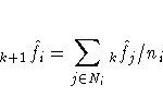
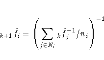
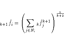
Cascaded density estimates are obtained by computing initial kernel density estimates and then, at each observation, taking the arithmetic mean, harmonic mean, or sum of the initial density estimates of the observations within the neighborhood. The cascaded density estimates can, in turn, be cascaded, and so on. Let $_{k}\hat{f}_i$ be the density estimate at x_i cascaded k times. For all types of cascading, $_{0}\hat{f}_i = \hat{f}_i$ .If the cascading is done by arithmetic means, then, for $k \geq 0$ ,

$_{k+1}{\hat{f}_i} = {\sum_{j\in{N_i}}{_k}{\hat{f}_j}}/{n_i}$

For harmonic means,

$_{k+1}{\hat{f}_i} = {( {\sum_{j\in{N_i}}{_k}{\hat{f}_j^{-1}} }/{n_i} ) }^{-1}$

and for sums,

$_{k+1}{\hat{f}_i} = {( \sum_{j\in{N_i}}{_k}{\hat{f}_j^{k+1}} ) }^{\frac{1}{k+2}}$

To avoid cluttering formulas, the symbol $\hat{f}_i$ is used from now on to denote the density estimate at x_i whether cascaded or not, since the clustering methods and significance tests do not depend on the degree of cascading.

Cascading increases the smoothness of the estimates with less computation than would be required by increasing the smoothing parameters to yield a comparable degree of smoothness. For population densities with bounded support and discontinuities at the boundaries, cascading improves estimates near the boundaries. Cascaded estimates, especially using sums, may be more sensitive to the local covariance structure of the distribution than are the uncascaded kernel estimates. Cascading seems to be useful for detecting very nonspherical clusters. Cascading was suggested by Tukey and Tukey (1981, p. 237). Additional research into the properties of cascaded density estimates is needed.

Chapter Contents
Previous
Next
Top