p-Value Adjustments

The MULTTEST Procedure

p-Value Adjustments

PROC MULTTEST offers p-value adjustments using Bonferroni, Sidak, Bootstrap resampling, and Permutation resampling, all with single-step or stepdown versions. In addition, Hochberg's (1988) and Benjamini and Hochberg's (1995) step-up methods are offered. The Bonferroni and Sidak methods are calculated from the permutation distributions when exact permutation tests are used with CA or PETO tests.

All methods but the resampling methods are calculated using simple functions of the raw p-values or marginal permutation distributions; the permutation and bootstrap adjustments require the raw data. Because the resampling techniques incorporate distributional and correlational structures, they tend to be less conservative than the other methods.

When a resampling (bootstrap or permutation) method is used with only one test, the adjusted p-value is the bootstrap or permutation p-value for that test, with no adjustment for multiplicity, as described by Westfall and Soper (1994).

Bonferroni

Suppose that PROC MULTTEST performs R statistical tests, yielding p-values p₁ , ... , p_R. Then the Bonferroni p-value for test r is simply Rp_r. If the adjusted p-value exceeds 1, it is set to 1.

If the unadjusted p-values are computed using exact permutation distributions, then the Bonferroni adjustment for p_r is p₁^*+ ... + p_R^*, where p_j^* is the largest p-value from the permutation distribution of test j satisfying $p_j^* \le p_r$ , or 0 if all permutational p-values of test j are greater than p_r. These adjustments are much less conservative than the ordinary Bonferroni adjustments because they incorporate the discrete distributional characteristics. However, they remain conservative in that they do not incorporate correlation structures between multiple contrasts and multiple variables (Westfall and Wolfinger 1997).

Sidak

A technique slightly less conservative than Bonferroni is the Sidak p-value (Sidak 1967), which is 1 - (1 - p_r)^R. It is exact when all of the p-values are uniformly distributed and independent, and it is conservative when the test statistics satisfy the positive orthant dependence condition (Holland and Copenhaver 1987).

If the unadjusted p-values are computed using exact permutation distributions, then the Sidak adjustment for p_r is 1-(1-p₁^*) ... (1- p_R^*), where the p_j^* are as described previously. These adjustments are less conservative than the corresponding Bonferroni adjustments, but they do not incorporate correlation structures between multiple contrasts and multiple variables (Westfall and Wolfinger 1997).

Bootstrap

The bootstrap method creates pseudo-data sets by sampling observations with replacement from each within-stratum pool of observations. An entire data set is thus created, and p-values for all tests are computed on this pseudo-data set. A counter records whether the minimum p-value from the pseudo-data set is less than or equal to the actual p-value for each base test. (If there are R tests, then there are R such counters.) This process is repeated a large number of times, and the proportion of resampled data sets where the minimum pseudo-p-value is less than or equal to an actual p-value is the adjusted p-value reported by PROC MULTTEST. The algorithms are described by Westfall and Young (1993).

In the case of continuous data, the pooling of the groups is not likely to recreate the shape of the null hypothesis distribution, since the pooled data are likely to be multimodal. For this reason, PROC MULTTEST automatically mean-centers all continuous variables prior to resampling. Such mean-centering is akin to resampling residuals in a regression analysis, as discussed by Freedman (1981). You can specify the NOCENTER option if you do not want to center the data. (In most situations, it does not seem to make much difference whether or not you center the data.)

The bootstrap method explicitly incorporates all sources of correlation, from both the multiple contrasts and the multivariate structure. The adjusted p-values incorporate all correlations and distributional characteristics.

Permutation

The permutation-style adjusted p-values are computed in identical fashion as the bootstrap adjusted p-values, with the exception that the within-stratum resampling is performed without replacement instead of with replacement. This produces a rerandomization analysis such as in Brown and Fears (1981) and Heyse and Rom (1988). In the spirit of rerandomization analyses, the continuous variables are not centered prior to resampling. This default can be overridden by using the CENTER option.

The permutation method explicitly incorporates all sources of correlation, from both the multiple contrasts and the multivariate structure. The adjusted p-values incorporate all correlations and distributional characteristics.

Stepdown Methods

Stepdown testing is available for the Bonferroni, Sidak, bootstrap, and permutation methods. The benefit of using stepdown methods is that the tests are made more powerful (smaller adjusted p-values) while, in most cases, maintaining strong control of the familywise error rate. The stepdown method was pioneered by Holm (1979) and further developed by Shaffer (1986), Holland and Copenhaver (1987), and Hochberg and Tamhane (1987).

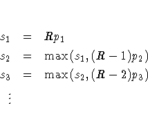
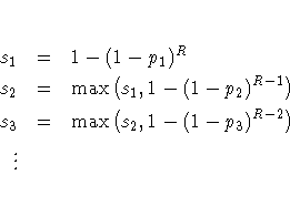
Suppose the base test p-values are ordered as p₁ < p₂ < ... < p_R. The Bonferroni stepdown p-values s₁, ... ,s_R are obtained from

$s_1 & = & Rp_1 \ s_2 & = & \max ( s_1 , (R-1) p_2 ) \ s_3 & = & \max ( s_2 , (R-2) p_3 ) \ \vdots & &$

As always, if any adjusted p-value exceeds 1, it is set to 1. The Sidak stepdown p-values are determined similarly:

$s_1 & = & 1 - (1 - p_1)^R \ s_2 & = & \max ( s_1 , 1 - (1 - p_2)^{R-1} ) \ s_3 & = & \max ( s_2 , 1 - (1 - p_3)^{R-2} ) \ \vdots & &$

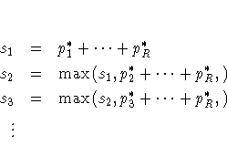
Stepdown Bonferroni adjustments using exact tests are defined as

$s_1 & = & p_1^*+ ... + p_R^* \ s_2 & = & \max ( s_1 , p_2^*+ ... + p_R^*, ) \ s_3 & = & \max ( s_2 , p_3^*+ ... + p_R^*, ) \ \vdots & &$

where the p_j^* are defined as before. Note that p_j^* is taken from the permutation distribution corresponding to the jth smallest unadjusted p-value. Also, any s_j greater than 1.0 is truncated to 1.0.

Stepdown Sidak adjustments for exact tests are defined analogously by substituting 1-(1-p_j^*) ... (1-p_R^*) for p_j^* + ... + p_R^*.

The resampling-style stepdown method is analogous to the preceding stepdown methods; the most extreme p-value is adjusted according to all R tests, the second-most extreme p-value is adjusted according to (R - 1) tests, and so on. The difference is that all correlational and distributional characteristics are incorporated when you use resampling methods. More specifically, assuming the same ordering of p-values as discussed previously, the resampling-style stepdown adjusted p-value for test r is the probability that the minimum pseudo-p-value of tests r, ... ,R is less than or equal to p_r.

This probability is evaluated using Monte Carlo, as are the previously described resampling-style adjusted p-values. In fact, the computations for stepdown adjusted p-values are essentially no more time-consuming than the computations for the nonstepdown adjusted p-values. After Monte Carlo, the stepdown adjusted p-values are corrected to ensure monotonicity; this correction leaves the first adjusted p-values alone, then corrects the remaining ones as needed. The stepdown method approximately controls the familywise error rate, and it is described in more detail by Westfall and Young (1993).

Hochberg

Assuming p-values are independent and uniformly distributed under their respective null hypotheses, Hochberg (1988) demonstrated that Holm's stepdown adjustments control the familywise error rate even when calculated in step-up fashion. Since the adjusted p-values are uniformly smaller for Hochberg's method than for Holm's method, the Hochberg method is more powerful. However, this improved power comes at the cost of having to make the assumption of independence.

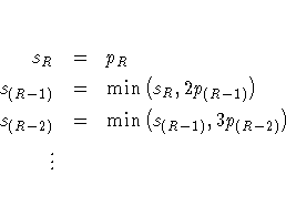
The Hochberg adjusted p-values are defined in reverse order as the stepdown Bonferroni:

$s_R & = & p_R \ s_{(R-1)} & = & \min ( s_R , 2 p_{(R-1)} ) \ s_{(R-2)} & = & \min ( s_{(R-1)} , 3 p_{(R-2)} ) \ \vdots & &$

False Discovery Rate

The FDR option requests p-values that control the "false discovery rate," described by Benjamini and Hochberg (1995). These adjustments are potentially much less conservative than the Hochberg adjustments; however, they do not necessarily control the familywise error rate. Furthermore, they are guaranteed to control the false discovery rate only with independent p-values that are uniformly distributed under their respective null hypotheses.

The FDR adjusted p-values are defined in step-up fashion, like the Hochberg adjustments, but with less conservative multipliers:

$s_R & = & p_R \ s_{(R-1)} & = & \min ( s_R , [R/(R-1)] p_{(R-1)} ) \ s_{(R-2)} & = & \min ( s_{(R-1)} , [R/(R-2)] p_{(R-2)} ) \ \vdots & &$

Chapter Contents
Previous
Next
Top