Survival Distribution Estimates for the Cox Model

The PHREG Procedure

Survival Distribution Estimates for the Cox Model

Two estimators of the survivor function are available: one is the product-limit estimate and the other is based on the empirical cumulative hazard function.

Product-Limit Estimates

Let C_i denote the set of individuals censored in the half-open interval [t_i , t_i+1), where t₀=0 and $t_{k+1}=\infty$ .Let $\gamma_l$ denote the censoring times in [t_i , t_i+1); l ranges over C_i . The likelihood function for all individuals is given by

${\cal L}=\prod_{i=0}^k \{ \prod_{l \in {\cal D}_i} ( [S_{0}(t_{i})]^{ {\rm exp... ... ) \prod_{l \in {\cal C}_i} [S_{0}(\gamma_{l}+0)]^{{\rm exp}(z'_{l}{\beta})} \}$

where D₀ is empty. The likelihood L is maximized by taking S₀(t)=S₀(t_i+0) for $t_{i}\lt t \leq t_{i+1}$ and allowing the probability mass to fall only on the observed event times t₁, , t_k. By considering a discrete model with hazard contribution $1-\alpha_{i}$ at t_i, you take $S_{0}(t_{i})=S_{0}(t_{i-1}+0)=\prod_{j=0}^{i-1} \alpha_j$ , where $\alpha_{0}=1$ . Substitution into the likelihood function produces

${\cal L}=\prod_{i=0}^k \{ \prod_{j \in {\cal D}_i } ( 1-\alpha_{i}^{{\rm exp}(z... ...d_{ l \in {\cal R}_{i}-{\cal D}_{i} } \alpha_{i}^{ {\rm exp}(z'_{l}{\beta})} \}$

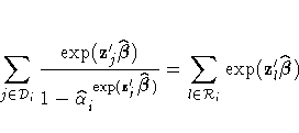
If you replace ${\beta}$ with $\hat{{\beta}}$ estimated from the partial likelihood function and then maximize with respect to $\alpha_{1}$ , , $\alpha_{k}$ , the maximum likelihood estimate $\hat{\alpha}_i$ of $\alpha_i$ becomes a solution of

$\sum_{ j \in {\cal D}_i } \frac { {\rm exp}(z'_{j}\hat{{\beta}}) } { 1-\hat{\a... ..._{j}\hat{{\beta}}) } } =\sum_{l \in {\cal R}_i } {\rm exp}(z'_{l}\hat{{\beta}})$

When only a single failure occurs at t_i, $\hat{\alpha}_i$ can be found explicitly. Otherwise, an iterative solution is obtained by the Newton method.

The estimated baseline cumulative hazard function is

$\hat{H}_{0}(t)=-{\rm log}(\hat{S}_{0}(t))$

where $\hat{S}_{0}(t)$ is the estimated baseline survivor function given by

$\hat{S}_{0}(t)=\hat{S}_{0}(t_{i-1}+0) =\prod_{j=0}^{i-1} \hat{\alpha}_{j} , t_{i-1} \lt t \leq t_{i}$

For details, refer to Kalbfleisch and Prentice (1980). For a given realization of the explanatory variables ${\xi}$ ,the product-limit estimate of the survival function at $Z={\xi}$ is

$\hat{S}(t,{\xi})= [\hat{S}_{0}(t)]^{\exp({\beta}'{\xi})}$

Empirical Cumulative Hazards Function Estimates

Let ${\xi}$ be a given realization of the explanatory variables. The empirical cumulative hazard function estimate at $Z={\xi}$ is

$\hat{\Lambda}(t,{\xi}) = \sum_{i=1}^n\int_{0}^t \frac{dN_{i}(s)}{\sum_{j=1}^nY_{j}(s)\exp(\hat{{\beta}}'(z_{j} - {\xi}))}$

The variance estimator of $\hat{\Lambda}(t,{\xi})$ is given by the following (Tsiatis 1981):

$& &\hat{var}\{n^{\frac{1}2}(\hat{\Lambda}(t,{\xi}) - \Lambda(t,{\xi}))\} \ & = ... ...i}))]^2} + \biggr. \biggl. H'(t,{\xi})\hat{V}(\hat{{\beta}})H(t,{\xi}) \biggr\}$

where $\hat{V}(\hat{{\beta}})$ is the estimated covariance matrix of $\hat{{\beta}}$ and

$H(t,{\xi}) = \sum_{i=1}^n\int_{0}^t \frac{\sum_{l=1}^n Y_{l}(s)(Z_{l}-{\xi})\ex... ...{\xi}))} {[\sum_{j=1}^n Y_{j}(s)\exp(\hat{{\beta}}'(z_{j} - {\xi}))]^2} dN_i(s)$

The empirical cumulative hazard function (CH) estimate of the survivor function for $Z={\xi}$ is

$\tilde{S}(t,{\xi})= \exp(-\hat{\Lambda}(t,{\xi}))$

Confidence Intervals for the Survivor Function

Let $\hat{S}(t,{\xi})$ and $\tilde{S}(t,{\xi})$ correspond to the product-limit (PL) and empirical cumulative hazard function (CH) estimates of the survivor function for $Z={\xi}$ , respectively. Both the standard error of log( $\hat{S}(t,{\xi})$ ) and the standard error of log( $\tilde{S}(t,{\xi})$ ) are approximated by $\tilde{\sigma}_{0}(t,{\xi})$ , which is the square root of the variance estimate of $\hat{\Lambda}(t,{\xi})$ ; refer to Kalbfleish and Prentice (1980, p. 116). By the delta method, the standard errors of $\hat{S}(t,{\xi})$ and $\tilde{S}(t,{\xi})$ are given by

$\hat{\sigma}_{1}(t,{\xi}) \dot{=} \hat{S}(t,{\xi})\tilde{\sigma}_{0}(t,{\xi}) ... ...tilde{\sigma}_{1}(t,{\xi}) \dot{=} \tilde{S}(t,{\xi})\tilde{\sigma}_{0}(t,{\xi})$

respectively. The standard errors of log[-log( $\hat{S}(t,{\xi})$ )] and log[-log( $\tilde{S}(t,{\xi})$ )] are given by

$\hat{\sigma}_{2}(t,{\xi}) \dot{=} \frac{- \tilde{\sigma}_{0}(t,{\xi})}{\log(\hat... ..._{2}(t,{\xi}) \dot{=} \frac{\tilde{\sigma}_{0}(t,{\xi})}{\hat{\Lambda}(t,{\xi})}$

respectively.

Let $z_{\alpha /2}$ be the upper $100(1-\frac{\alpha}2)$ percentile point of the standard normal distribution. A $100(1-{\alpha})\%$ confidence interval for the survivor function $S(t,{\xi})$ is given in the following table.

Method CLTYPE Confidence Limits

LOG PL $\exp[\log(\hat{S}(t,{\xi})) +- z_{\frac{\alpha}2}\tilde{\sigma}_{0}(t,{\xi})]$

LOG CH $\exp[\log(\tilde{S}(t,{\xi})) +- z_{\frac{\alpha}2}\tilde{\sigma}_{0}(t,{\xi})]$

LOGLOG PL $\exp\{-\exp[\log(-\log(\hat{S}(t,{\xi}))) +- z_{\frac{\alpha}2}\hat{\sigma}_{2}(t,{\xi})]\}$

LOGLOG CH $\exp\{-\exp[\log(-\log(\tilde{S}(t,{\xi}))) +- z_{\frac{\alpha}2}\tilde{\sigma}_{2}(t,{\xi})]\}$

NORMAL PL $\hat{S}(t,{\xi})+- z_{\frac{\alpha}2}\hat{\sigma}_{1}(t,{\xi})$

NORMAL CH $\tilde{S}(t,{\xi})+- z_{\frac{\alpha}2}\tilde{\sigma}_{1}(t,{\xi})$

Chapter Contents
Previous
Next
Top

Method	CLTYPE	Confidence Limits
LOG	PL	$\exp[\log(\hat{S}(t,{\xi})) +- z_{\frac{\alpha}2}\tilde{\sigma}_{0}(t,{\xi})]$
LOG	CH	$\exp[\log(\tilde{S}(t,{\xi})) +- z_{\frac{\alpha}2}\tilde{\sigma}_{0}(t,{\xi})]$
LOGLOG	PL	$\exp\{-\exp[\log(-\log(\hat{S}(t,{\xi}))) +- z_{\frac{\alpha}2}\hat{\sigma}_{2}(t,{\xi})]\}$
LOGLOG	CH	$\exp\{-\exp[\log(-\log(\tilde{S}(t,{\xi}))) +- z_{\frac{\alpha}2}\tilde{\sigma}_{2}(t,{\xi})]\}$
NORMAL	PL	$\hat{S}(t,{\xi})+- z_{\frac{\alpha}2}\hat{\sigma}_{1}(t,{\xi})$
NORMAL	CH	$\tilde{S}(t,{\xi})+- z_{\frac{\alpha}2}\tilde{\sigma}_{1}(t,{\xi})$