Chapter Contents

Previous

Next

Getting Started

In the following example, PROC PRINQUAL uses the MTV method. Suppose that the problem is to linearize a curve through three-dimensional space. Let

where X = -1.00, -0.98, -0.96, ... , 1.00.

These three variables define a curve in three-dimensional space. The GPLOT procedure is used to display two-dimensional views of this curve. These data are completely described by three linear components, but they define a single curve, which could be described as a single nonlinear component.

PROC PRINQUAL is used to attempt to straighten the curve into a one-dimensional line with a continuous transformation of each variable. The N=1 option in the PROC PRINQUAL statement requests one principal component. The TRANSFORM statement requests a cubic spline transformation with nine knots. Splines are curves, which are usually required to be continuous and smooth. Splines are usually defined as piecewise polynomials of degree n with function values and first n-1 derivatives that agree at the points where they join. The abscissa values of the join points are called knots. The term "spline" is also used for polynomials (splines with no knots) and piecewise polynomials with more than one discontinuous derivative. Splines with no knots are generally smoother than splines with knots, which are generally smoother than splines with multiple discontinuous derivatives. Splines with few knots are generally smoother than splines with many knots; however, increasing the number of knots usually increases the fit of the spline function to the data. Knots give the curve freedom to bend to more closely follow the data. Refer to Smith (1979) for an excellent introduction to splines. For another example of using splines, see Example 65.1 in Chapter 65, "The TRANSREG Procedure."

One component accounts for 71 percent of the variance of the untransformed data, and after 50 iterations, over 98 percent of the variance of the transformed data is accounted for by one component (see Figure 53.2). The algorithm did not converge with 50 iterations, so more iterations may be needed for this problem.

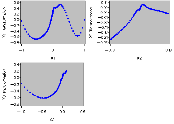
PROC PRINQUAL creates an output data set (which is not displayed) that contains both the original and transformed variables. The original variables have the names X1, X2, and X3. Transformed variables are named TX1, TX2, and TX3. All observations in the output data set have _TYPE_='SCORE', since the CORRELATIONS option is not specified in the PROC PRINQUAL statement. The GPLOT procedure uses this output data set and displays the nonlinear transformations of all three variables and the nearly one-dimensional scatter plot (see Figure 53.3 and Figure 53.4).

PROC PRINQUAL tries to project each variable on the first principal component. Notice that the curve in this example is closer to a circle than to a function from some views (see the plot of X3 vs. X2 in Figure 53.1) and that the first component does not run approximately from one end point of the curve to the other (see Figure 53.4). Since the curve has these characteristics, PROC PRINQUAL linearizes the scatter plot by collapsing the scatter around the principal axis, not by straightening the curve into a single line. PROC PRINQUAL would straighten simpler curves.

The following statements produce Figure 53.1 through Figure 53.4:

   * Generate a Three-Dimensional Curve;
   data X;
      do X = -1 to 1 by 0.02;
         X1 =      X ** 3;
         X2 = X1 - X ** 5;
         X3 = X2 - X ** 6;
         output;
      end;
      drop X;
   run;

   goptions goutmode=replace nodisplay;
   %let opts = haxis=axis2 vaxis=axis1 frame cframe=ligr;
   * Depending on your goptions, these plot options may work better:
   * %let opts = haxis=axis2 vaxis=axis1 frame;

   proc gplot data=X;
      title;
      axis1 minor=none label=(angle=90 rotate=0)
            order=(-1 to 1);
      axis2 minor=none order=(-1 to 1);
      plot X1*X2 / &opts name='prqin1';
      plot X3*X2 / &opts name='prqin2' vreverse;
      plot X1*X3 / &opts name='prqin3';
      symbol1 color=blue;
   run; quit;

   goptions display;
   proc greplay nofs tc=sashelp.templt template=l2r2;
      igout gseg;
      treplay 1:prqin1 2:prqin2 3:prqin3;
   run; quit;

   * Try to Straighten the Curve;
   proc prinqual data=X n=1 maxiter=50 covariance;
      title 'Iteratively Derive Variable Transformations';
      transform spline(X1-X3 / nknots=9);
   run;

   * Plot the Transformations;
   goptions nodisplay;
   proc gplot;
      title;
      axis1 minor=none label=(angle=90 rotate=0);
      axis2 minor=none;
      plot TX1*X1 / &opts name='prqin4';
      plot TX2*X2 / &opts name='prqin5';
      plot TX3*X3 / &opts name='prqin6';
      symbol1 color=blue;
   run; quit;

   goptions display;
   proc greplay nofs tc=sashelp.templt template=l2r2;
      igout gseg;
      treplay 1:prqin4 2:prqin6 3:prqin5;
   run; quit;

   * Plot the Straightened Scatter Plot;
   goptions nodisplay;
   proc gplot;
      axis1 minor=none label=(angle=90 rotate=0)
            order=(-1 to 1);
      axis2 minor=none order=(-1 to 1);
      plot TX1*TX2 / &opts name='prqin7';
      plot TX3*TX2 / &opts name='prqin8' vreverse;
      plot TX1*TX3 / &opts name='prqin9';
      symbol1 color=blue;
   run; quit;

   goptions display;
   proc greplay nofs tc=sashelp.templt template=l2r2;
      igout gseg;
      treplay 1:prqin7 2:prqin8 3:prqin9;
   run; quit;

Chapter Contents

Previous

Next

Top

Copyright © 1999 by SAS Institute Inc., Cary, NC, USA. All rights reserved.