Computational Method

Chapter Contents

The SURVEYREG Procedure

Computational Method

For a stratified clustered sample design, observations are represented by an n ×(p+2) matrix

(w, y, X) = (w_hij, y_hij, x_hij)

where

w denotes the sampling weight vector
y denotes the dependent variable
X denotes the design matrix. (When an effect contains only classification variables, the columns of X corresponding to this effect contain only 0s and 1s; no reparameterization is made.)
h = 1, 2, ... , H is the stratum number with a total of H strata
i = 1, 2, ... , n_h is the cluster number within stratum h, with a total of n_h clusters
j = 1, 2, ... , m_hi is the unit number within cluster i of stratum h, with a total of m_hi units
p is the total number of parameters (including an intercept if the INTERCEPT effect is included in the MODEL statement)
$n=\sum_{h=1}^H \sum_{i=1}^{n_h} {m_{hi}}$ is the total number of observations in the sample

Also, f_h denotes the sampling rate for stratum h. You can use the TOTAL= option or the RATE= option to input population totals or sampling rates. See the section "Specification of Population Totals and Sampling Rates" for details. If you input stratum totals, PROC SURVEYREG computes f_h as the ratio of the stratum sample size to the stratum total. If you input stratum sampling rates, PROC SURVEYREG uses these values directly for f_h. If you do not specify the TOTAL= option or the RATE= option, then the procedure assumes that the stratum sampling rates f_h are negligible, and a finite population correction is not used when computing variances.

Regression Coefficients

PROC SURVEYREG solves the normal equations ${X'WX}{\beta}={X'Wy}$ using a modified sweep routine that produces a generalized (g2) inverse (X'WX)^- and a solution (Pringle and Raynor 1971)

$\hat{{\beta}}={(X'WX)^-X'WY}$

where W is the diagonal matrix constructed from WEIGHT variable values.

For models with class variables, there are more design matrix columns than there are degrees of freedom (DF) for the effect. Thus, there are linear dependencies among the columns. In this case, the parameters are not estimable; there is an infinite number of least-squares solutions. PROC SURVEYREG uses a generalized (g2) inverse to obtain values for the estimates. The solution values are not displayed unless you specify the SOLUTION option in the MODEL statement. The solution has the characteristic that estimates are 0 whenever the design column for that parameter is a linear combination of previous columns. (Strictly termed, the solution values should not be called estimates.) With this full parameterization, hypothesis tests are constructed to test linear functions of the parameters that are estimable.

Variance Estimation

PROC SURVEYREG uses the Taylor series expansion theory to estimate the covariance-variance matrix of the estimated regression coefficients (Fuller 1975). Let

${r=y-X\hat{{\beta}}}$

where the (h,i,j)th element is r_hij. Compute 1×p row vectors

$e_{hij} &=& w_{hij} r_{hij} x_{hij} \ e_{hi\cdot}&=& \sum_{j=1}^{m_{hi}}e_{hij} \ \bar{e}_{h\cdot\cdot} &=& \frac1{n_h}\sum_{i=1}^{n_h}e_{hi\cdot}$

and calculate the p×p matrix

$G=\frac{n-1}{n-p} \sum_{h=1}^H { \frac{n_h(1-f_h)}{n_h-1} \sum_{i=1}^{n_h} { (e_{hi\cdot}-\bar{e}_{h\cdot\cdot})' (e_{hi\cdot}-\bar{e}_{h\cdot\cdot}) } }$

PROC SURVEYREG computes the covariance matrix of ${\beta}$ as

${\hat V = (X'WX)^-G(X'WX)^-}$

Testing Effects

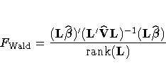
For each effect in the model, PROC SURVEYREG computes an L matrix such that every element of $L{\beta}$ is estimable; the L matrix has the maximum possible rank associated with the effect. To test the effect, the procedure uses the Wald F statistic for the hypothesis $H_{0}\colon L {\beta}= 0$ . The Wald F statistic equals

$F_{\rm Wald} = \frac{(L\hat{{\beta}})' (L'\hat{V} L)^{-1} (L\hat{{\beta}}) } {{\rm rank}(L)}$

with numerator degrees of freedom equal to rank(L) and denominator degrees of freedom equal to the number of clusters minus the number of strata (unless you have specified the denominator degrees of freedom with the DF= option in the MODEL statement; see the section "Denominator Degrees of Freedom"). It is possible that the L matrix cannot be constructed for an effect, in which case that effect is not testable. For more information on how the matrix L is constructed, see the discussion in Chapter 12, "The Four Types of Estimable Functions."

Multiple R-squared

PROC SURVEYREG computes a multiple R-squared for the weighted regression as

R² = 1-[(SS_error)/(SS_total)]

where SS_error is the error sum of squares in the ANOVA table

SS_error = r'Wr

and SS_total is the total sum of squares

${\rm SS_{total}} = \{ {{y'Wy} & {if no intercept}\ {y'Wy}- \displaystyle {(\su... ...{hij}y_{hij})^2 / w_{\cdot \cdot \cdot} } & {if there is an intercept} } .$

where w_··· is the sum of the sampling weights over all observations.

Root Mean Square Errors

PROC SURVEYREG computes the square root of mean square errors as

$\sqrt{\rm MSE} = \sqrt{n {\rm SS_{error}} / (n-p) w_{\cdot \cdot \cdot} }$

where w_··· is the sum of the sampling weights over all observations.

Design Effect

If you specify the DEFF option in the MODEL statement, PROC SURVEYREG calculates the design effects for the regression coefficients. The design effect of an estimate is the ratio of the actual variance to the variance computed under the assumption of simple random sampling.

DEFF = [ Variance under the Sample Design/ Variance under Simple Random Sampling]

Refer to Kish (1965, p.258). PROC SURVEYREG computes the numerator as described in the section "Variance Estimation". And the denominator is computed under the assumption that the sample design is simple random sampling, with no stratification and no clustering.

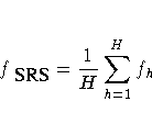
To compute the variance under the assumption of simple random sampling, PROC SURVEYREG calculates the sampling rate as follows. If you specify both sampling weights and sampling rates (or population totals) for the analysis, then the sampling rate under simple random sampling is calculated as

f_SRS = n / w_···

where n is the sample size and w_··· (the sum of the weights over all observations) estimates the population size. If the sum of the weights is less than the sample size, f_SRS is set to zero. If you specify sampling rates for the analysis but not sampling weights, then PROC SURVEYREG computes the sampling rate under simple random sampling as the average of the stratum sampling rates.

$f_{{ \rm SRS}} = \frac{1}H \sum_{h=1}^H f_h$

If you do not specify sampling rates (or population totals) for the analysis, then the sampling rate under simple random sampling is assumed to be zero.

f_SRS = 0

Sampling Rate of the Pooled Stratum from Collapse

Assuming that PROC SURVEYREG collapses single-unit strata h₁, h₂, ... , h_c into the pooled stratum, the procedure calculates the sampling rate for the pooled stratum as

$f_{{Pooled Stratum}}= \{ {0 & {if any of } f_{h_l}=0 { where } l=1, 2, ... , ... ...{l=1}^c n_{h_l}f_{h_l}^{-1} )^{-1} \sum_{l=1}^c n_{h_l}} & {otherwise} } .$

Contrasts

You can use the CONTRAST statement to perform custom hypothesis tests. If the hypothesis is testable in the univariate case, the Wald F statistic for $H_{0}: L {\beta}= 0$ is computed as

$F_{\rm Wald} = \frac{({L_{\rm Full}}\hat{{\beta}})' ({L_{\rm Full}}'\hat{V} {L_{\rm Full}})^{-1} ({L_{\rm Full}}\hat{{\beta}}) } {{\rm rank}(L)}$

where L is the contrast vector or matrix you specify, ${\beta}$ is the vector of regression parameters, $\hat{{\beta}}={(X'WX)^-X'WY}$ , $\hat{V}$ is the estimated covariance matrix of $\hat{{\beta}}$ , rank(L) is the rank of L, and L_Full is a matrix such that

-: L_Full has the same number of columns as L
-: L_Full has full row rank
-: the rank of L_Full equals the rank of the L matrix
-: all rows of L_Full are estimable functions
-: the Wald F statistic computed using the L_Full matrix is equivalent to the Wald F statistic computed using the L matrix with any row deleted that is a linear combination of previous rows

If L is a full-rank matrix, and all rows of L are estimable functions, then L_Full is the same as L. It is possible that L_Full matrix cannot be constructed for contrasts in a CONTRAST statement, in which case the contrasts are not testable.

Chapter Contents
Previous
Next
Top