Computational Methods
Four methods of estimation can be specified in the PROC VARCOMP
statement using the METHOD= option. They are described in the
following sections.
The Type I Method
This method (METHOD=TYPE1) computes the Type I sum of squares for
each effect, equates each mean square involving only random effects
to its expected value, and solves the resulting system of equations
(Gaylor, Lucas, and Anderson 1970). The  matrix
is computed and adjusted in segments whenever memory is not
sufficient to hold the entire matrix.
matrix
is computed and adjusted in segments whenever memory is not
sufficient to hold the entire matrix.
The MIVQUE0 Method
Based on the technique suggested by Hartley, Rao, and LaMotte
(1978), the MIVQUE0 method (METHOD=MIVQUE0) produces unbiased
estimates that are invariant with respect to the fixed effects of
the model and that are locally best quadratic unbiased estimates
given that the true ratio of each component to the residual error
component is zero. The technique is similar to TYPE1 except that the
random effects are adjusted only for the fixed effects. This affords
a considerable timing advantage over the TYPE1 method; thus, MIVQUE0
is the default method used in PROC VARCOMP. The  matrix is computed and adjusted in segments whenever memory is not
sufficient to hold the entire matrix. Each element (i,j) of the
form
matrix is computed and adjusted in segments whenever memory is not
sufficient to hold the entire matrix. Each element (i,j) of the
form
-
SSQ(Xi'MXj)
is computed, where
-
M = I-X0(X0'X0)-X0'
and where X0 is part of the design matrix for the fixed
effects, Xi is part of the design matrix for one of the random
effects, and SSQ is an operator that takes the sum of squares of the
elements. For more information refer to Rao (1971, 1972) and
Goodnight (1978).
The Maximum Likelihood Method
The Maximum Likelihood method (METHOD=ML) computes
maximum-likelihood estimates of the variance components; refer to
Searle, Casella, and McCulloch (1992). The computing algorithm
makes use of the W-transformation developed by Hemmerle and Hartley
(1973). The procedure uses a Newton-Raphson algorithm, iterating
until the log-likelihood objective function converges.
The
objective function for METHOD=ML is  , where
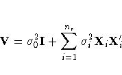
and where  is the residual variance, nr is the number of random
effects in the model,
is the residual variance, nr is the number of random
effects in the model,  represents the variance components,
Xi is part of the design matrix for one of the random
effects, and
represents the variance components,
Xi is part of the design matrix for one of the random
effects, and
-
r = y- X0 (X0' V-1 X0)- X0' V-1 y
is the vector of residuals.
The Restricted Maximum Likelihood Method
The Restricted Maximum Likelihood Method (METHOD=REML) is similar to
the maximum likelihood method, but it first separates the likelihood
into two parts: one that contains the fixed effects and one that
does not (Patterson and Thompson 1971). The procedure uses a
Newton-Raphson algorithm, iterating until convergence is reached for
the log-likelihood objective function of the portion of the
likelihood that does not contain the fixed effects. Using notation
from earlier methods, the objective function for METHOD=REML is
 .Refer to Searle, Casella, and McCulloch (1992) for additional
details.
.Refer to Searle, Casella, and McCulloch (1992) for additional
details.
Copyright © 1999 by SAS Institute Inc., Cary, NC, USA. All rights reserved.