The subject of chaos has attracted a lot of attention over the last few decades, but most of the examples that have become popular are visual. The more proper term for this class of phenomena is that they are non-linear dynamic systems, and in fact there is an acoustic component to them.
However, the main characteristics of the field are usually introduced with a specific type of recursive equation with a non-linear component, with the simplest being the Logistic Map or Verhulst map. This equation has been used to model an animal population, for instance, depending on another variable such as the number of predators.
In terms of the equation, the non-linearity is a simple x2 which doesn’t seem very complicated. However, when you scale the non-linearity with a multiplier called r, and use the equation iteratively, then certain kinds of behaviour start to emerge with large numbers of iterations.
By iteratively, we mean that the next value x(n+1) is derived from the current value x(n) by the following equation, which behaves as follows depending on the value of r.
LOGISTIC MAP (Verhulst)x(n+1) = r . x(n) . [1 - x(n)]
converges to zero (r < 1)
converges to a fixed value (1 > r < 3)
bifurcates into 2, 4, 8
1st chaotic region (r = 3.57)
bifurcates into periodic functions
2nd chaotic region
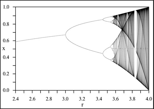
The Logistic Map in the region of r above 2.4
This portion of the map shows a convergence to a fixed value between r = 2.4 and 3.0, at which point a series of what are called period doublings occur. This means the values oscillate between two values. This is followed by more period doublings to four and 8. After that (at r = 3.57) there is a totally chaotic region, with moments of sudden periodicity, as the r value approaches 4.
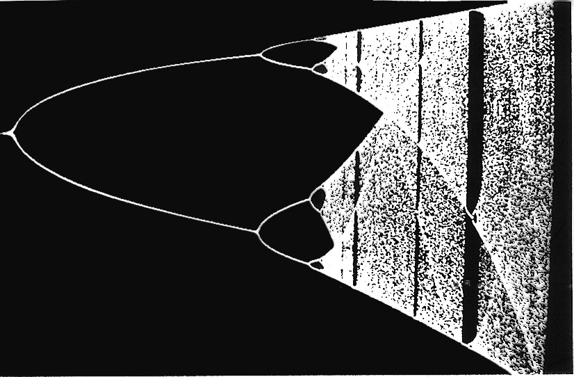
Here is another version that I programmed for pixels on a screen, starting at r = 3 with the first period doubling. Another aspect of this behaviour is that there is self-similarity at deeper levels of the pattern.
Finally, here is a mapping of the Logistic Map onto granular synthesis, specifically the frequency of the grain. As r ascends you will first hear the region where the values converge to zero, followed by a dramatic shift where they converge to a fixed frequency that continues to rise, followed by the period doublings and the chaotic region with flashes of periodicity.
logistic map projected onto granular synthesis, sweeping r from 0 to 4
PSEUDO PHASE SPACE
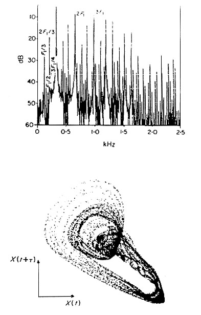
Pseudo-phase space refers to a two-dimensional mapping of a sound where, instead of the X axis being time, and the Y axis being the amplitude, the Y axis is a delayed version of the X axis (similar to Lissajous figures on an oscilloscope). A periodic function will look like a closed loop since its phase pattern is periodic. However, with non-linearity, we will find a period doubling in the patterm as shown here.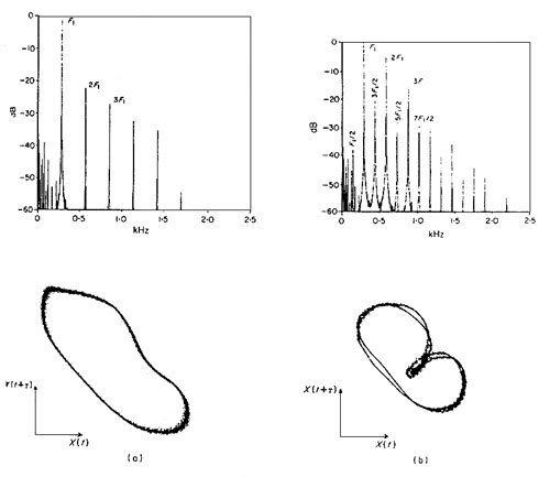
(a) periodic oscillation in pseudo phase space (lower) and corresponding spectrum (upper); (b) same system with higher gain, showing period doubling
This diagram shows period tripling in a clarinet multiphonic (from V. Gibiat, "Phase space representations of acoustical musical signals," Journal of Sound and Vibration, 123(3), 1988.
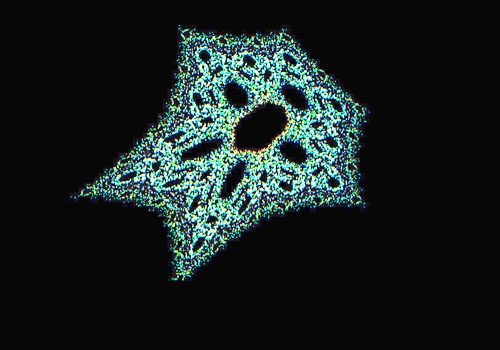
Gingerbread Man Distribution
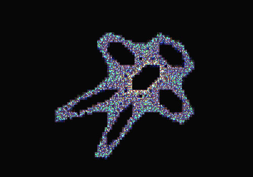
We now go to a purely mathematical function which doesn't model anything in the real world, but whose standard representation is pseudo-phase space. That is, the next X value depends on the current Y value and the next Y value is the current X (hence the "delay"). The non-linearity is the absolute value of the current X value indicated with the slashes in the equation:
x(n+1) = 1 - y(n) + / x(n) / The similarity to a gingerbread man obviously provides its name, but values cluster around certain points and totally avoid others. When magnified you can see areas of self-similarity. The mapping onto grains is now with the frequency bandwidth from which specific values are chosen. The cycle repetition gets rather tedious, so we also show an enveloped version. The next graphics are a typical result when one scales the non-linearity by a factor of A.y(n+1) = x(n)
Mapping onto the frequency of grains:
x(n+1) = 1 - x(n-1) + / x(n) / FREQ(n+1) = CENTRE FREQUENCY + x(n+1) . FREQUENCY RANGE
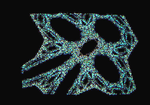
with scaled non-linearity:x(n+1) = 1 - x(n-1) + A . / x(n) /
gingerbread man algorithm mapped to grain frequency, first with constant global amplitude, then envelopedgingerbread man algorithm mapped to start position of a vocal sample
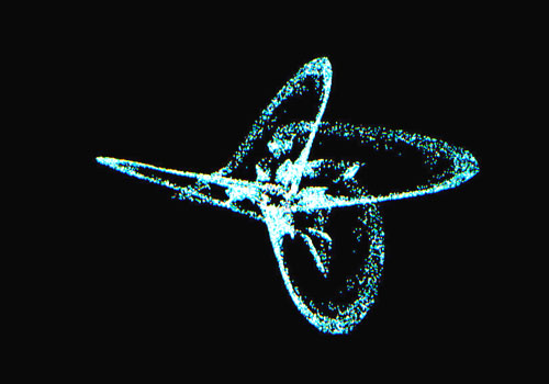
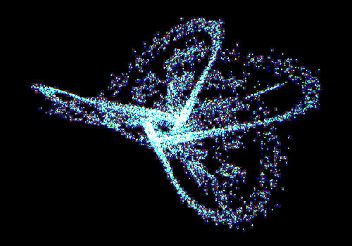
Next we extend the equation with scaled previous sample (three dimensional?) similar to a digital filter.
x(n+1) = 1 - y(n) + A. / x(n) / - B . x(n-1) y(n+1) = x(n)
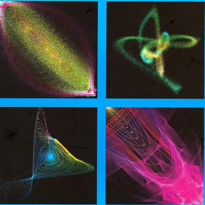
Pseudo-phase space maps for flute tone
(upper left) high note with noise; (upper right) low note; (lower right) low note synthesized by fractal interpolation; (lower left) short trumpet note
from Gordon Monro & Jeff Pressing, "Sound visualization using embedding: The art and science of auditory autocorrelation," Computer Music Journal, 22(2), 1998, pp. 20-34.
home