A. Filters and Equalizers. Filters
and Equalizers process sound in the frequency domain,
and as a result they are used to modify the spectrum
of the sound, that is, its frequency content, and hence its timbre. If you
are unfamiliar with the concepts and representations of
spectrum, it would be good to review the second Vibration module.
The main difference between filters and equalizers are that
filters only attenuate (i.e. reduce) certain
frequencies in the spectrum, whereas equalizers can either boost
or attenuate the strength of particular frequency
bands of the spectrum. A hybrid form of these models is called
a shelf filter, which is somewhat of a misnomer, as it
can boost or attenuate all of the high frequencies (a high
shelf) or the low frequencies (a low shelf) above or below a
certain frequency, respectively.
Another class of equalizer – and clearly the most powerful –
is called a parametric equalizer, the term parametric
referring to the fact that all parameters of an equalizer are
controllable simultaneously. In the analog studio, these were
quite complex units, whereas today you are likely to begin
with a parametric plug-in which has all of the functions
described here available together, so it is best if you
understand all of them.
The simplest filters are the high-pass and low-pass
filters which can only attenuate frequencies below or above
what is called the cut-off frequency. Here we already
have a potential point of confusion, so memorize this formula:
a high-pass filter passes the highs and
attenuates the lows
a
low-pass filter passes the lows and attenuates the highs
Where the confusion arises is that when you
want to get rid of some low frequencies, as shown below, you
need a high pass filter; keep in mind that the term “pass”
refers to not affecting that range and passing
those frequencies through unchanged.
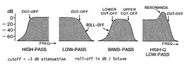
At the left we have the
high-pass and low-pass filters. They have two variables, the
cut-off frequency which is where the signal is
attenuated by 3 dB (that is, where the attenuation is
regarded as significant), and the roll-off which is
the slope of the filter’s response beyond the
cut-off. In other words, the term “cut” is not an accurate
description of the filter’s action as it implies removing
something (true), but in a clean and precise manner (not
possible). All filters, whether analog of digital, cannot
eliminate, for instance, all frequencies below exactly 100
Hz, which would require a rectangular response.
Instead,
all frequencies below the cut-off of a high-pass filter are
gradually attenuated according to the slope of the
roll-off. Because it can be thought of as a slope, the units
are decibels per octave, in other words, it
specifies how much attenuation there is with each octave. It
might help to think of the slope of a highway, the grade,
expressed as a percentage. With a roll-off of 12 dB/oct and
a cutoff of 100 Hz (which is attenuated 3 dB by definition),
the attenuation at 50 Hz (an octave lower) would be 3 + 12 =
15 dB.
The
important distinction is that the larger the roll-off value,
the more precisely it distinguishes between the desired
frequencies that remain (i.e. are passed) and those which
are attenuated. Today, digital filters typically have slopes
of 16, 24 or more (e.g. 48 dB/octave) which is more than
enough to isolate a frequency band cleanly. The limiting
factor to having an extremely steep slope is that it adds phase
distortion to the sound, hence the impossibility of
having a rectangular cut.
In analog filters, the roll-off is fixed by the circuitry
and cannot be changed. In digital filters, the roll-off is
calculated as variables in an equation. Therefore,
you can only select a desired roll-off and switch to
it, as opposed to the cut-off frequency which can be swept
up or down continuously at will, an interactive ability that
is aurally very effective for hearing the changes in the
spectrum.
Also, this type of sweep often produces an aurally
interesting way of introducing a sound into a mix, starting
with a high cutoff in a high-pass filter and lowering it
gradually, or vice versa with a low-pass filter, an
alternative to the conventional fade-in. A good
digital filter will not have clicks when the cut-off
is swept, so be careful with any that produce this kind of
artifact.
The bandpass filter, shown above,
is the combination (quite literally) of these two filters,
the high-pass and low-pass. It is controlled by two
cut-offs, low and high, with the distance between them
referred to as the passband. Because there are two
variables in a bandpass filter (plus the roll-off), a
digital application will have to decide if there are two
separate controls, and if so, which ones.
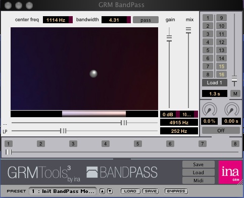
One choice that works well is centre frequency and bandwidth
(to borrow terms from the Equalizer). If the control surface
is a two-dimensional window with an X-Y axis, then this
double choice could work well for a mouse moving around the
space (for instance, as found in the GRM Tools approach, as
shown below).
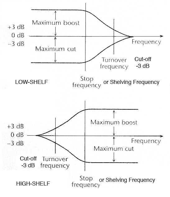
As briefly mentioned above, the shelf filter is a
hybrid between a low-pass (or high-pass) filter and an
equalizer. The difference is the lack of a continuous
roll-off. All frequencies below the cut-off or turnover
frequency in a low shelf filter are either
boosted or attenuated (that is, + or - gain in
decibels). Once the gain is decided, that is the gain for all
frequencies below what is called the stop frequency or shelving
frequency.
Something similar happens with a high shelf, except
that the gain is for frequencies above the cut-off
or turnover frequency. In practice, the shelf filter seems
cruder than the bandpass, particularly when it is
attenuating. In terms of low frequencies, the high-pass
filter will progressively eliminate them, whereas a low
shelf filter will merely lower them in intensity. Presumably
the difference is whether removing or simply lowering those
frequencies is the desired goal. Use of the shelf filter to
boost all highs or lows should be done carefully, if at all.
Equalizers (used to EQ a
sound) come in many variations, the main one being how many
bands are available, the more the better, in general.
It is useful to think of an equalizer as a set of filters,
where each band has a fixed bandwidth, usually
defined in octaves and fractions thereof. However, unlike
the filters we've considered, gain can be applied to boost
or attenuate each band.
A third-octave bandwidth, meaning 3 separate bands
per octave (with a total of between 24 and 30 bands to
control) is a standard. When we study the ear’s resolving
power for frequencies in a spectrum, called the critical
bandwidth (that will be deal with in the second Vibration module), we will
find that it is a little less than a quarter of an octave,
so the 1/3 octave equalizer comes close to
controlling exactly the range of frequencies that we can
hear separately in a spectrum.
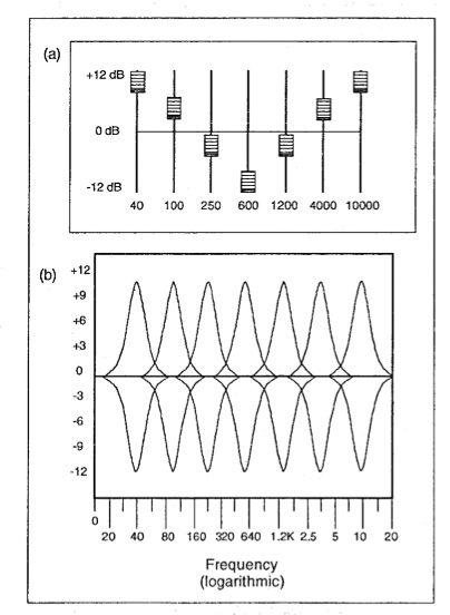
The diagram below, if taken literally, would not be a very
good equalizer as it only has 7 bands to cover a 9-octave
range of frequencies, even though they are distributed on a
logarithmic frequency scale. So, each band covers over an
octave, which might make it easy to use in a car audio
system, but it is ill-suited for audio design work. The
saving grace of the diagram is that it is easier to see what
is going on than, say, with a 24-band equalizer.
The controls on an equalizer, for each band, are the choice
of centre frequency and the gain, plus or
minus, which is continuously variable up to or down to a
maximum, here shown as +/- 12, but more typically +/- 15 or
20. In general it is the “curved” shape of this set
of gains that is most effective, rather than the maximum
gain. In fact, so much gain can be cumulatively applied with
an equalizer that the sound will distort and/or be
unpleasant to our ears, particularly if the boost is in the
1-4 kHz range where the ear is most sensitive.
Multi-band
equalizer (a)
and its frequency response pattern (b)
Parametric Equalizer. A
parametric equalizer makes all of its variables
controllable, namely:
Centre Frequency (CF) in Hz or kHz
Gain in + or - dB
Bandwidth as the ratio Q where Q =
Centre Frequency / Bandwidth
If
the last controllable parameter (Q) were actually
bandwidth, it would be difficult to use because of the
logarithmic nature of frequency. For instance, from 100 to
200 Hz is an octave, and the bandwidth is 100 Hz; the
octave from 1 kHz to 2 kHz represents a bandwidth of 1000
Hz. So, if we kept the bandwidth constant at 100 Hz, and
swept the centre frequency from 100 Hz to 1 kHz, we’d go
from a very large bandwidth to a very narrow one
perceptually, with resulting inconsistency in how the
result would sound. Admittedly we could keep it constant
as a ratio with an interval of, say, 1/3 octave,
but that isn’t very easy to specify in general.
Therefore, by creating the unitless ratio of Q,
being the ratio between the centre frequency and the
bandwidth, we keep the actual bandwidth comparable at all
centre frequencies. The usual range of Q is from 1 to 10,
or higher in digital versions, which can also be thought
of as a range of bandwidths from being equal to the centre
frequency to being 1/10 of it for Q = 10.
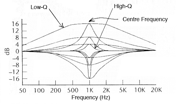
Narrow bandwidths, with a Q above 5 or 6, may be narrow
enough that, when applied to broadband sounds, a spectral
pitch will emerge, somewhat similar to a vocal formant
which is a narrow resonance region that helps to identify
a vowel. The diagram below shows the range of Q from low
(i.e. broad bandwidth) to high (i.e. very narrow
bandwidth) at different gain levels for clarity.
In general, the Q factor should be judged carefully by ear
to being just enough to give the sound more focus and
presence, but not so much as to be annoyingly intrusive
(since the auditory system is very focused on picking up
such resonance regions). This type of boost in the 2-3 kHz
region will give speech added presence and clarity, as
demonstrated later.
Parametric
equalizer frequency response for various values of Q
A useful subset of the parametric equalizer is
the notch filter which provides a very narrow
attenuation of a specific frequency. The most common use is
for eliminating a 60 Hz hum (or 50 Hz in Europe). Similarly,
a peak filter offers a single band similar to the
parametric model.
B. Interface representations of filters
and equalizers.
Low-pass, high-pass and bandpass filters.
These include a range of graphic controls with virtual knobs
and sliders, and a visual frequency response diagram – which
is useful, but don't take the shapes too literally. Some
allow the processing shapes to be stored for later use, and
most have some kind of bypass function to allow the
effect to be turned off and on, which is very useful for
comparisons to the original, or in the case of multiple
functions being used at the same time, to check the effect
of each one separately and as a set. Although this is a
limited set that compares 3 and 4 plug-ins, you should be
able to find similar features in other ones that you have
available.
Many
plug-ins offer several filter/EQ functions that are combined
in one interface, but despite it being in software, the
companies don't bother to change the parameter names on the
graphics, so you really need to know your parameters to use
them efficiently.
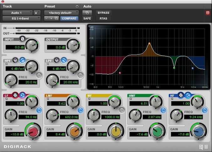
This
simple 4-band plug-in has the typical high-pass
and low-pass curves as selected on bands 1 &
4. It allows you to sweep the white ball for each
cut-off with a fixed roll-off.
The middle knob shows the cut-off frequency and
allows control via the knob as a slider.
If the result is weak, the vertical slider at
right allows for gain control. Bypass switches at
the bottom.
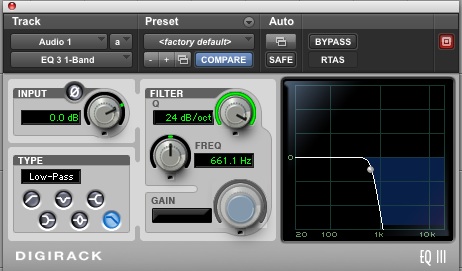
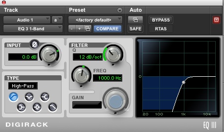
These
are the standard ProTools single-band filters.
Note the icons for all the modes at the lower
left.
On the right what is actually the roll-off
is incorrectly called Q and offers a choice from 6-24
dB/octave or more.
The cut-off frequency can be swept with the knob
as a slider or by dragging the white dot.
(click to enlarge)
This
is the standard parametric processor in Audition
which includes all of the standard processes,
including high-pass (HP) and low-pass (LP) at the
far left and right respectively.
A choice of cut-offs is offered, plus gain control
at the left. Because this is a digital filter, the
roll-off can be chosen from 6 dB/oct up to 48
dB/oct. However, note that all frequency changes
in real time, such as the cut-offs, will result in
clicks as they are moved.
This
is the standard bandpass model in GRM Tools, which
comes in both a mono and stereo version. Once you
know how it works, the stereo version is excellent
for treating left and right channels independently
which will likely provide an interesting spatial
spread to the timbre.
The x-axis is centre frequency and the y-axis is
bandwidth, with numerical values at the top, so
both low-pass and high-pass functions are neatly
combined in a single gesture within the mouse
paradigm. The actual values in Hz for the two
cut-offs are indicated in small windows to the
right of the individual manual controls for them.
The other functions are standard for all GRM
functions and can be consulted in the
documentation.
High and low shelf
filters. These are the filters used to boost or
attenuate all low or high frequencies past a certain point.
The
top diagram shows the low and high shelf filters
(left and right) attenuated, and the bottom
diagram shows them boosted (probably inadvisable),
both in bands 1 and 4. The top two knobs control
gain and cut-off frequency respectively. Note the
shelving pattern beyond those points and compare
it to the high-pass and low-pass filters above.
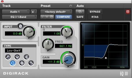
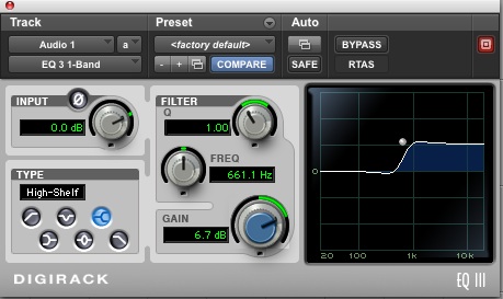
The
top diagram shows the standard ProTools
single-band filter in low shelf mode with
attenuation, and the bottom diagram shows the high
shelf with positive gain.
Note the stirrup-shaped icons for these. The top
slider knob controls the steepness of the curve
(called the Q); the cut-off frequency and gain are
controlled with the other two slider knobs.
(click to enlarge)
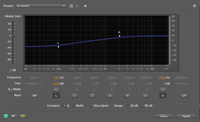
This
diagram shows Audition’s standard parametric
processor in low and high shelf mode together
(marked L and H, not to be confused with HP and LP
which are nearby).
The lows are being attenuated and highs boosted.
This example uses the “gentle slope” switch
(above the L and H).
(click to enlarge)
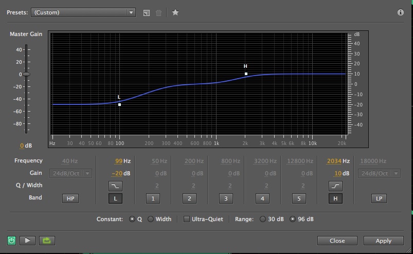
This
diagram shows Audition’s standard parametric
processor in low and high shelf mode together
(marked L and H, not to be confused with HP and LP
which are nearby).
The lows are being attenuated and highs boosted.
This example uses the “steep slope” switch
(above the L and H).
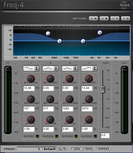
Peak and notch filters.
These are subsets of the general parametric model, offering
one or two controllable bands.
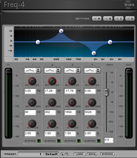
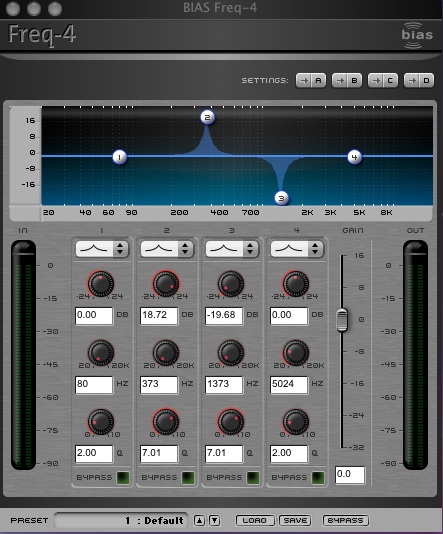
The top diagram shows two bands
(left and right) with a boost and attenuation
respectively, with a low Q, i.e. broad
bandwidth. The bottom diagram shows them with a
high Q, i.e. narrow bandwidth, corresponding to
what otherwise might be called peak and notch
modes. All three knobs are in use to control
(top to bottom) gain, centre frequency, and Q.
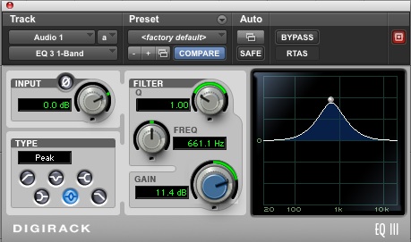
The top diagram shows the standard
ProTools 1-band filter in peak mode with a boost
(that could be changed to attenuation with
negative gain) and choice of Q, in this case 1
which is quite broad.
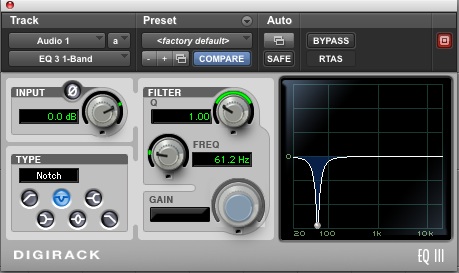
The bottom diagram shows the specialized
narrow-band notch filter where the gain is
maximized negatively, the Q value determines the
bandwidth, and the FREQ slider knob controls the
centre frequency. Note the different icons for
each of these.
(click to enlarge)
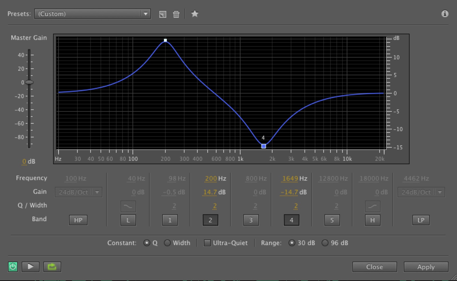
This diagram shows Audition’s
standard parametric processor used with two
bands simultaneously (marked 2 and 4). The lows
are being boosted in the first band and the
highs attenuated in the second, but with a low Q
of 2, i.e. a broad bandwidth. Note that each
band can be turned off and on.
(click to enlarge)
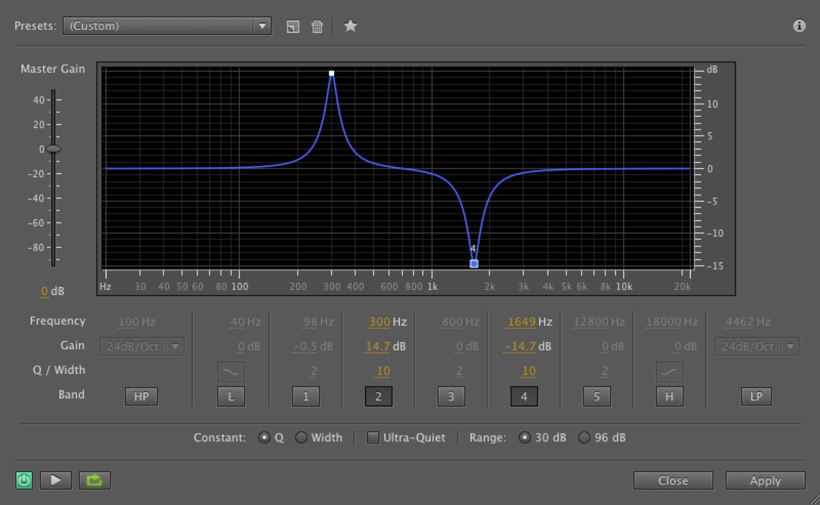
This diagram shows Audition’s
standard parametric processor used with two
bands simultaneously (marked 2 and 4). The lows
are being boosted in the first band and the
highs attenuated in the second, but with a high
Q of 10 (the max), i.e. a narrow bandwidth. Note
that each band can be turned off and on.
Full Parametric
Equalizers. The Audition examples shown above
were all taken from its full parametric plug-in, so any of
the various processes could be added together. With
ProTools, the 7-band parametric could look intimidating, as
shown next, despite being colour-coded, so again, it's best
to learn each format thoroughly before using it.
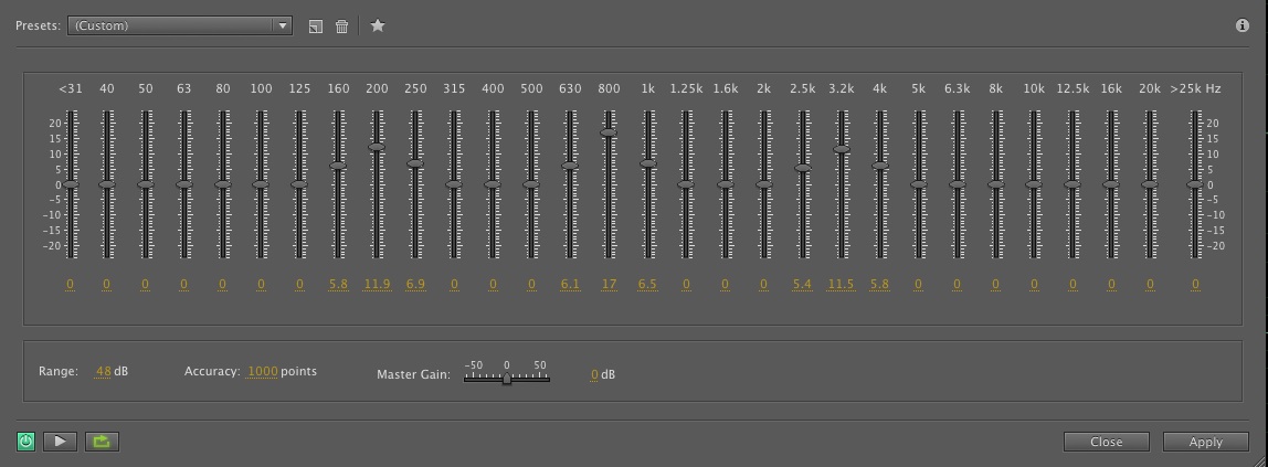
Third-octave Equalizers.
Unlike the interfaces for analog filters and
parametric equalizers, the interface paradigm for the
third-octave equalizer has not changed significantly in
its migration into the digital domain. Each band of
filters is represented by a vertical line where the
vertical dimension represents gain above or below
a zero point (i.e. where no gain is applied). The bands
themselves are identified by the centre frequency
based on the international standard of 1 kHz and
its octaves and sub-octaves. For a third-octave equalizer,
there will be two additional bands between each of those
octaves.
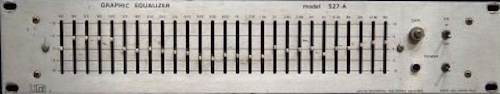
Traditional analog 27-band graphic equalizer
Within a “mouse paradigm” where only one value can
be adjusted at a time, a serious problem arises for this
kind of processor – how to control its many variables
efficiently. With the analog version, some skill in using
both sets of fingers to control multiple bands
simultaneously provided a certain kind of performability
for dynamic changes. However, the implied norm for its use
was for a fixed setting: once the controls were put in
place, they stayed there. The same applies to most
plug-ins, but steps can be taken for dynamic changes as
discussed below.
We have already noted a significant extension to the
“mouse paradigm” with GRM Tools’ Bandpass model where two
variables in the x-y plane can be controlled by a the
mouse on a small screen. However, unless you have an
extremely steady hand to move a mouse smoothly, dynamic
changes can sound jerky. GRM Tools solved this problem
with the ability to interpolate between presets
with a ramp whose speed can be specified in a small box
below the presets (and stored with the preset). For
filters and equalizers, among others, these smooth ramps
(which can be continuously changed over time with multiple
presets) offer an improvement over the analog version in
terms of performability.
Third-octave equalizer in Audition (click
to enlarge)
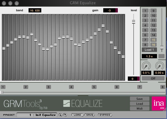
The GRM Graphic Equalizer follows the standard
paradigm with a few differences. The EQ curve can be
“drawn” by running the mouse over the surface – but not
too quickly – to trace a general curve. Then, each band
can be modified by dragging the gain of an individual band
up or down (with the corresponding centre frequency and
gain indicated at the top). Any configuration can be
stored as a preset. However, note that there is no zero
line, and in fact the gain could be lowered to zero,
unlike an analog equalizer.
Rather unusually for GRM, the default group of presets are
not particularly useful, some being quite flat. An unusual
configuration for any equalizer is to have alternate
bands up and down, or every third one up – the octave
configuration. Given the 1/3 oct bandwidth, a spectral
pitch will be heard even with noisy sounds, since
any of these configurations resembles resonances in an air
space. Musically, a third of an octave is a major third,
and every second band is an minor sixth
apart, so some kinds of tonal sounding “chords” can be
created.
Tip: The GRM Equalizer default presets have some
of these alternating band combinations, but since the
lower gains go to zero, they do not cross-fade very
smoothly, as the loudness drops in between presets.
Raising the low gains to a higher value will correct this
issue.
C. Circuits for using
processors. In the analog studio where everything
had to be patched (i.e. connected) together, creating a
circuit or signal path was absolutely
fundamental as well as very flexible and open-ended.
Today, most signal paths are hidden or assumed, and at
least one, the parallel circuit is much more
difficult to create and use. Before we embark below on
practical studio experiments, it would be useful to know
about some of these types of circuits, where your
challenge will be how to create them with your own
equipment and software.
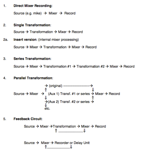
1. A direct recording refers to whatever
route a signal takes from the microphone to a sound
file, where "mixer" might refer to a simple level
control. If you are importing a soundfile, then this
step is not necessary.
2. A single
transformation, or the "insert" version 2a, puts some
kind of processor in between the source and its
subsequent saved output. In the analog studio there
was a subtle distinction about whether the
transformation happened before it arrived at the mixer
or after. In digital processing, the standard plug-in
as illustrated above, is the equivalent to this form
of single transformation, and is usually provided on
every track.
3. Likewise, if the software allows multiple plug-ins,
the assumption is that they are in a series
configuration, that is, the output of the first goes
into the second, and so on. When using such multiples,
it is good to keep in mind that each process must be
compatible with the previous one. If the first is a
filter that removes low frequencies, for instance,
they can’t be part of the processing in the second
process.
4. The parallel circuit, in the analog
tradition, relied on being able to split the signal
into exact copies, that is, multiple versions, with no
loss of strength. This was accomplished with a special
patch bay wiring called a bridge or “multi” with
several connections joined together electrically to
avoid signal loss. With one input, all the other
connections could be outputs, and the multi could be
patched to another for even more outputs. These were
then routed to independent processors and back into
the mixer to be combined. The beauty and simplicity of
this setup was that all signals were heard and
processed in real time, and could be mixed in stereo
formats at will.
Today, auxiliary circuits
can be used on a DAW or mixer for a real-time version
of the parallel circuit, but they are more complicated
to set up for beginners. Both a real-time and
non-realtime version will be described in the studio
demo’s below as a kind of submix. All auxiliary
circuit, whether analog or digital, allow the signal
to be sent to the processing unit either independently
of the playback level of the original (called pre,
meaning before the playback level), or at a level that
depends on the playback level (called post,
meaning after the playback level and therefore
dependent on it).
5. A feedback circuit is one where the signal
is fed back and mixed with the original, but only
where there’s enough of a delay involved that it
doesn’t immediately go into distortion, as indicated
in the second example above where the recording
machine playback or a digital delay is used. It can
also be called recirculation because a loop
has been set up. The other requirement is a sensitive
control over the feedback levels, which can
increase the signal exponentially; that is, small
changes become large ones. Most of the examples
of this approach will be described in the modules on
Time Delays. However, feedback with filters at modest
levels can make them sound more like resonators.
D. Introduction to
Digital Filters using Waveguides. The topic of
digital filters from an engineering perspective is very
complex, involving differential equations in their
design, and not all of them will be related to sound
design. However, it is still useful to consider some
simple examples of what are called 1st and 2nd order
filters that can be modelled using a short delay
line also known as a waveguide. Basically,
the waveguide is a memory array of n samples that are
continuously stored and replaced once full. Therefore
the contents of the waveguide reflect the most recent
values of the waveform.
With these filter algorithms, only the previous sample,
referred to as x(n-1), or the second previous sample,
x(n-2), are used, so the delay line is very short, and
in fact can be implemented with one or two variables
that temporarily store these previous values.
The samples themselves are usually multiplied by a gain
coefficient, often labelled g, and are combined
with the direct signal which goes from the input, x(n),
to the output y(n) in these diagrams. The 1st order
examples are called that because they use only the
previous sample, whereas the 2nd order use the
2nd previous sample in the calculation.
Introducing the concepts of delay lines and waveguides
here will prepare the way for their use in longer lines
for our presentation of phasing (with short
delays) and echo and reverb models (with long
delays) in later modules.
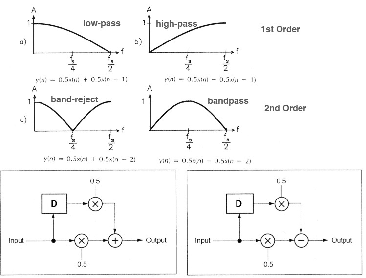
These
diagrams show four basic filters in terms of their frequency response,
equations and delay line circuits, from top to bottom.
Here you will see that the two 1st order models describe
the familiar low-pass and high-pass
filters. The left-hand graphic circuit model shows that
the input signal at left goes into a delay line D, gets
scaled by .5 and is combined (the + sign) with the
direct signal which is also multiplied by .5 to form the
output signal at the right.
This is a formal way of saying we are averaging
the current sample with the previous sample, since
averaging involves adding two numbers together and
dividing by two. However, in the frequency domain, we
have learned that frequency is the rate of change of
phase, with higher frequencies showing a more rapid
change of phase. When we average out those rapid peaks,
we are essentially filtering them out, hence the
low-pass effect.
Also note that the delay for the
low-pass filter, D, is 1 sample (i.e. first order), and
for the band-reject filter D = 2, the second previous
sample, but otherwise the circuit is the same. Although
simple, it turns out that these filters are not very
useful because the slope of their roll-off is
very gentle. Note also that the “zero” of the
filter moves from the half sampling rate (Fs) for the
first-order filter, to half that with the second-order
filter (hence the term band reject).
For the two filters at the right, a similar process
occurs, but instead of averaging the adjacent samples,
we subtract them from each other. Since low
frequencies move slowly in terms of phase, adjacent
samples will show little difference in value, and
therefore when samples are subtracted, a small value
will result. As noted, the 1st order version is a high-pass
filter, and the second order is a very simple bandpass
filter. Note the location of the zeroes in these
filters, as well as their “poles” where the
output amplitude is highest. Higher orders in filter
design using more scaled previous samples would be
needed to improve the roll-off.
Finally, we should note that these filters are called
FIR filters, Finite Impulse Response, because
they settle to zero quickly, lacking any feedback in the
circuit that would prolong them.
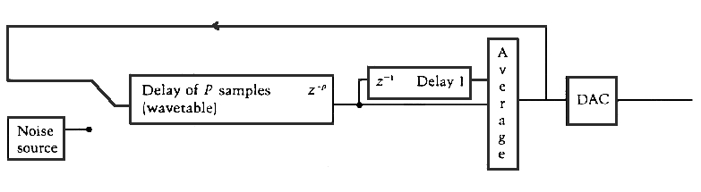
However, when we model the resonances
on a string (as in the first Vibration
module), there is feedback because of the waves
are reflected at both ends. Therefore, in the simple Karplus-Strong
model of the string, as shown below, there is an
averaging function shown as a delay of one sample
(engineers refer to the length of the delay line with a
z with an exponent of -p where p is the
length of the waveguide) in order to average the value.
This acts as the simple low-pass filter shown
above. Because of the recirculation of the values in the
waveguide, even the simplest low-pass averaging filter
will be effective because the filtering process happens
again and again.
The K-S model feeds its values back into the delay line
(whose length corresponds to that of the string),
consistent with the standing wave phenomenon
that is created in a real string. However, what we are
“processing” with a string is the initial energy applied
to it, namely the pluck, which is modelled by
filling up the waveguide with random numbers,
but once filled, adding no more, similar to a single
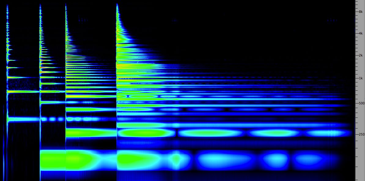
pluck. Note the aural realism of the result including
the decay of the sound lengthening with the length of
the string/waveguide.
Karplus-Strong
delay line resonator
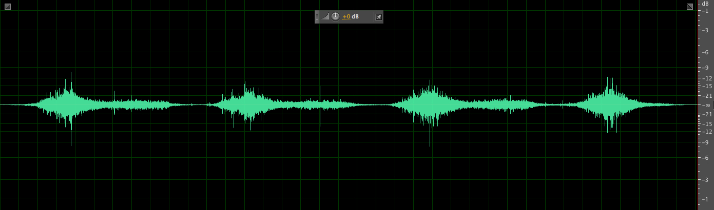
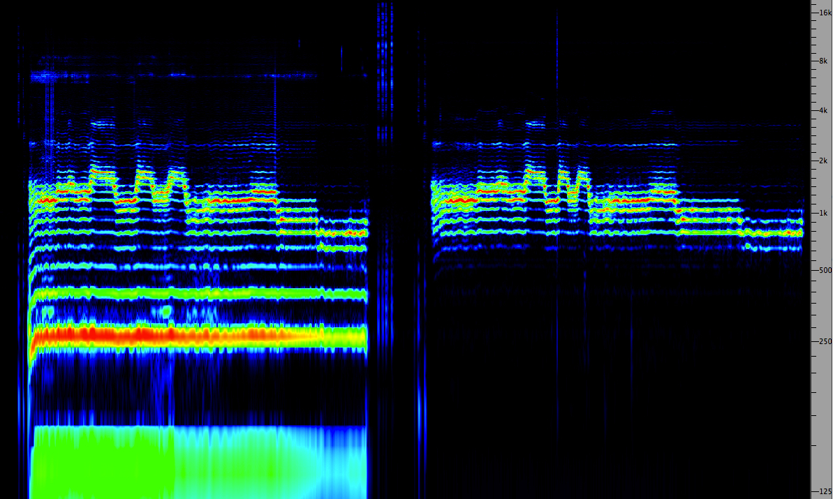
Four
plucks of the string model, with the
waveguide length doubled each time and the
resulting spectrogram
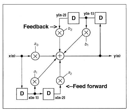
To complete this brief survey of
digital filters, we have two more diagrams, the one at
left showing an Infinite Impulse Response filter
(IIR) which incorporates both the feed forward
function that we saw above, that is, adding two previous
input samples, x(n-1) and x(n-2), to the direct signal,
as well as a feedback function that recirculates
two of the previous output samples, y(n-1) and y(n-2).
Note the gain values called coefficients are the
various a, b values. This feedback function creates the
“ringing” behaviour of theoretically infinite
repetitions, similar to the various forms of audio
feedback we will encounter later. Careful control
over the feedback level will affect how long it lasts.
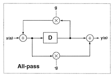
The right hand diagram shows an all-pass
filter which means that all frequencies are passed
equally, that is, with the same gain, but there are
predictable phase shifts in certain frequencies.
Keep in mind that the two most salient
points in this topic are that:
manipulation of the time domain in
terms of delay samples affects the frequency
domain (a characteristic of microsound)
filters can exhibit resonating
behaviour when feedback is involved
Q. Try this review quiz to test your
comprehension of the above material (not including Digital
Filters), and perhaps to clarify some distinctions you may
have missed. Note that a few of the questions may have
"best" and "second best" answers to explain these
distinctions.
E. Studio Demo's and Personal Projects.
With some exceptions, we will not be referencing
specific equipment in these demo’s, but for you to
replicate them (definitely a good idea), you will need to
find equivalent solutions with whatever software you have
available. However, we are recommending that you use both
a waveform editor with whatever plug-ins it is
equipped with for processing, and a DAW (digital
audio workstation) for assembling and mixing your files.
Some waveform editors, such as Audition, include a small
mixing module where multiple tracks can be combined. This
can be useful for test mixes and submixes, i.e. where you
combine multiple versions of your sounds into a mix that
can be bounced into a cumulative file.
a. Using filters and
equalizers. In starting a project or experiment, the
so-called raw recording you intend to use will
likely need to be edited and cleaned up. Some users will
prefer to keep the original recording intact, for future
reference, whereas others might already delete any
extraneous sounds and adjust levels (particularly
when the record level is low) with the editor.
After you’ve made those choices, the next stage of
clean-up might be to use a filter to get rid of
unwanted low frequencies, for instance. Even if you end up
using only a subset of the entire source soundfile (see
the personal experiments below), it is a good idea to have
all of it cleaned up in this manner first, so you won’t
have to do it again if you go back to the original (and
forget how you cleaned it up).
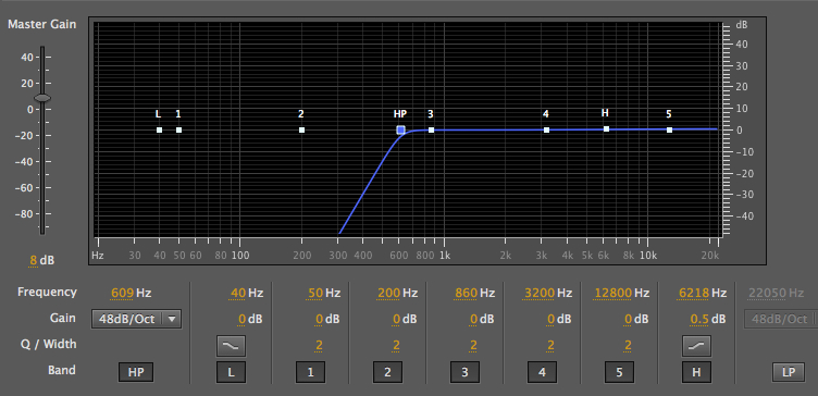
1. Using a
high-pass filter.
Original scything recording
with wind noise
Source:
WSP Canada 32 take 10
Click on the link to see the exact high-pass
filter settings in Audition. Note that the high-pass
filter (HP) has a cut-off frequency of 609 Hz, and that
the roll-off is set to the maximum value, 48 dB/octave
which cleanly reduces the low frequency portion of the
spectrum. Since low frequencies tend to have high
amplitude waveforms, the difference in the before and
after waveforms are telling. It’s actually unusual to be
able to see such processing differences at the waveform
level (we will rely on the spectrogram after this), but
low-frequency noise is always quite visible. Given that so
much energy was removed from the signal, note that a
Master Gain of 8 dB was added to the filtering. This could
have be done later, but was easy to predict during the
processing setup.
The reason this example works so well is that, in terms of
the spectrum, the “desired” component of the sound, the
scything sound, occupies the region above 500 Hz, and the
wind occupies everything below that. Therefore, they can
be easily separated. However, if those components
overlapped significantly, a compromise would have to be
made as to how much to attenuate the desired sound in
order to minimize the unwanted component.
Rolling off the low frequencies is also
sometimes desirable in the spoken voice. Roughly speaking,
the male voice will likely go down to around 100 Hz, and
the female voice to 200 Hz. However, room resonances
(called eigentones)
will boost the low frequencies in a voice, as does a
typical amplification of the voice in that space which for
the moment we are limiting to medium-sized spaces which
are not large enough (or empty enough) to produce
significant reverberation.
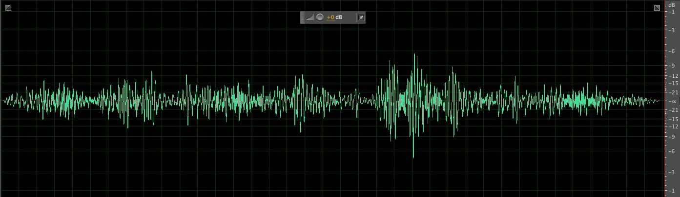
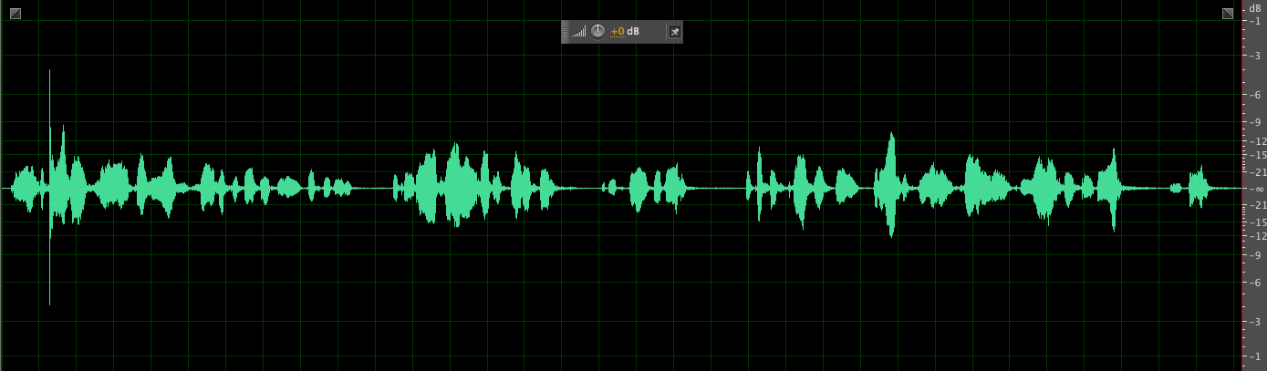
British Columbia elder Herb George speaking place
names in his native language, first filtered below 400
Hz, then opened up fully
Rolling off the lows with a voice recorded
indoors will have the effect of making it sound farther
away and possibly outdoors, particularly if ambience is
added. It is surprising how seldom this simple
processing is done in media contexts, particularly radio
dramas. The scene is clearly set outdoors, but the
voices are clearly studio recorded with noticeable low
frequency resonances. Why do listeners (not to mention
the producers) not find this illogical?
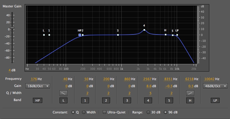
The recording is of a female professor
giving a public introduction, and is of medium quality
(we’ve all heard much worse). A parametric equalizer in
Audition was used to give the voice more presence,
first by rolling off the low frequencies with the
high-pass filter, with a cut-off of 176 Hz (there is
little energy in the female voice below 200 Hz, but the
room itself was somewhat boomy, so this was needed). A
roll-off of 18 dB/oct was chosen to not attenuate the
lows too much (which would have made the voice sound
more distant and less resonant).
Then in EQ band 4 there’s a classic EQ
boost of 8.6 dB around 2.5 kHz (where significant
formant
information is located in the vowels, hence the boosted
clarity and presence). Note that the Q value is
5 to give it some bandwidth but not too much. Finally a
low-pass filter (LP) rolls off the top octave above 10
kHz quite steeply. A modest Master Gain of +8 dB is
added. Although the result does not repair all of the
faults of the original, it certainly makes it clearer
and easier to listen to. However, this EQ pattern is so
commonly used, it would make sense to save it as a
preset for inevitable future use.
Note that the plosive
consonant “p” in the word “department” was very
prominent in the original near the start, which is
typical of the standard positioning of the mike in front
of the speaker’s face (instead of slightly to the side).
The air expelled by the plosive consonants, e.g. p, b,
t, goes straight into the mic and is heard as a
broadband noise, mainly low frequency, but if strong
enough, some mid-range energy as well. It is clearly
seen in the waveform near the start. As a micro-editing
exercise, the so-called “popping p” was also excised
from the EQ’d version with the editor, ensuring that no
phase discontinuity was added. The result at the bottom
right is somewhat more acceptable.
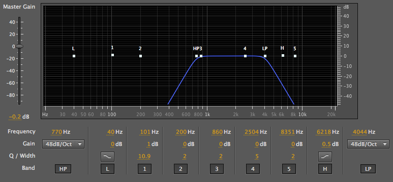
3.
Using a strongly limited bandpass filter.
Original voice recording with
multiphonics (Yves Candau)
The recording is of a male singer with a
remarkable ability to sing what are called multiphonics.
These are harmonics created by adjusting resonances
within the vocal tract as controlled by the tongue.
The pattern that was used in Audition strongly
attenuated the frequencies below 770 Hz and above 4
kHz, leaving the harmonics present that were more than
two octaves above the fundamental.
4. Using strong bandpass filter and
parametric equalization.
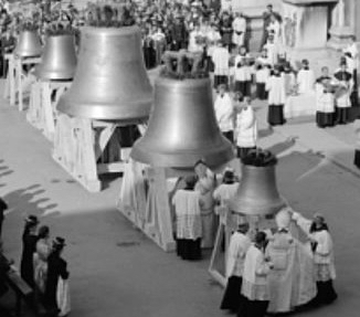
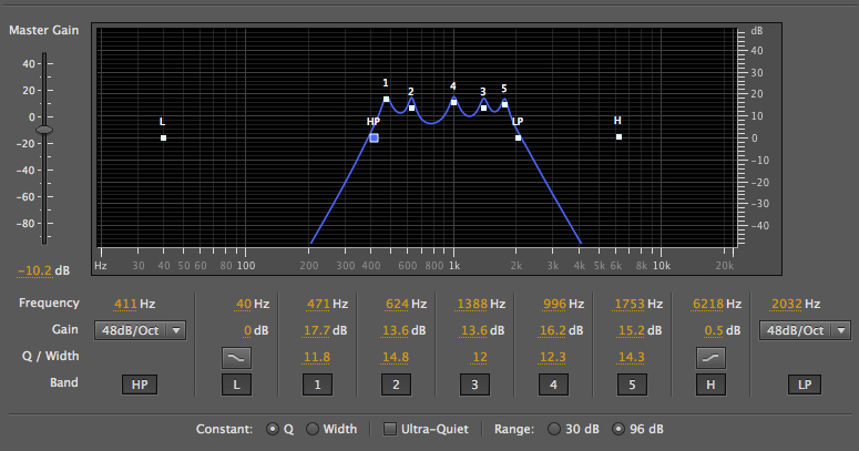
Salvator Mundi bell,
Salzburg
Source: WSP Eur 28 take 2
The recording is of the very large solo
bell known as “Salvator Mundi” from the Salzburg
cathedral, weighing 14,000 kg, and rung only on feast
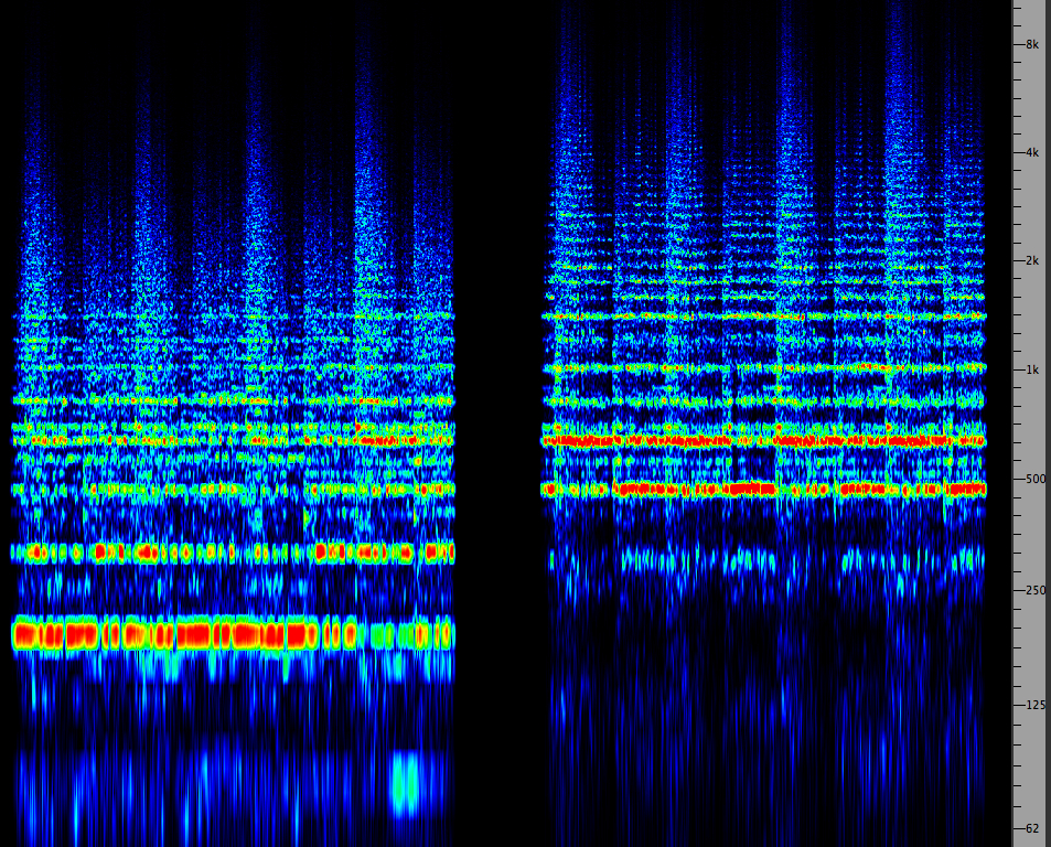
days. The bandpass that was used in Audition strongly
attenuated the frequencies below 411 Hz and above 2
kHz, leaving the partials present that were more than
two octaves above the fundamental. Then – strictly by
ear, but also using the spectrogram – all 5 parametric
bands were tuned to specific frequencies in the
spectrum, giving them boosts from 13.6 dB to 17.7 dB.
Note that the Q values are around 12-14, meaning quite
narrow bandwidths. Given this amount of boosting, the
Master Gain was dropped by 10 dB to prevent overload.
Although this kind of result is aurally interesting by
itself, it may also be used in a mix with the original
so that a smooth transition between the original and
one enhanced in these partials is possible. Also, this
harmonic cluster could be treated as secondary
source material from which to derive octave
transpositions, granular time stretching and
convolution based transformations, among others.
b) Personal Studio Experiment No. 1
Based on the examples and information covered so
far, you should be able to embark on some interesting
experiments to work with actual sounds. The approach
we’re taking here is the classic sound object
exercise that has proved valuable over the
decades as a technique for honing your listening
skills, as well as advancing your technical and
creative abilities.
It is based on using just a few sounds and maximizing
their transformations, and as such it’s a good
way to try out a lot of sound processing techniques.
But what you’ll probably find out is that the more you
manipulate a sound, the more you learn about it, and
hopefully at some point along the way, the sound
itself will lead you in some creative directions
you’ve never imagined.
The process is entirely open-ended, and you should be
mainly guided by your ears, but also by relying on
what you have learned. Here are some steps that might
help you to get started.
1. Select a soundfile that you think
would be interesting to work with, and make sure it
is cleaned up, editing out extraneous material,
correcting any low levels, and filtering out
frequencies such as the lows that may not be
desirable. Keep in mind that computer speakers, and
even headphones, are not the best way to determine
the presence of lows. Save the result as your
reference soundfile (which we will refer to as the source).
2. If there are some specific parts of your source
that are also interesting, highlight those in your
editor and save the selection to a new file
(or copy and paste). If it has an abrupt start or
end, use the amplitude tools your software provides
to fade-in the start, and fade-out
the end, even if it’s a very short fade. You can
also try looping this selection to hear whether it
works well in repetition, and make any adjustments
to improve the break between the end and start. You
can make more such short excerpts, but
you’ll probably not have time to explore them all.
3. Start transposing your source or the
excerpts up and/or down, depending on which range is
strongest in the source. Although you can use any
size of pitch transposition, doing it by octaves has
several advantages. First, you can quickly get to
the “end” of what is going to be usable in either
directions. Remember the old saying: you don’t know
you’ve gone too far until you’ve gone too far.
Secondly, octave combinations always work well
aurally, even if there are not actual pitches
involved.
Ideally you’ll make two versions of each
transposition, one that maintains the same
duration, and one that multiplies it by two for each
transposition down an octave, or halves it for the
upward transpositions, similar to playing a tape at
half or double its normal speed. For the downward
transpositions, you may need to boost the
level each time as it will drop off, particularly
towards the lower frequencies.
Very important: when you “Save as” each
version, make sure you give it a file name that
reflects the process, e.g. “Bell-1oct” and
“Bell-1octSt” where St might be your reminder that
it was stretched in length (or compressed for the
upper ones). In general, lower transpositions work
best and having some very long stretches may also be
useful.
A
variation on this approach is where you bandpass filter
a part of the spectrum of your source, particularly
if it is broadband. Listen to the source for
differences in texture and character in the upper,
middle and lower parts of the spectrum, perhaps with
the aid of a bandpass filter. It is often true that
a “part” of the sound in the frequency domain may be
more useful to you than the entire range. And when
these bands of frequency are transposed, the result
will also be cleaner and more useful for combining
in a mix. At some point you might want to EQ
the sound as well, similar to what we did with the
bell above.
As you transpose and/or stretch the sound, notice
how the character of it changes, or what aural image
it creates. Some sounds, like water, tend to stay
recognizable as water no matter what transposition
you make, probably since there are such a wide
variety of water sounds in the soundscape. Others
will have a different affect or image in different
ranges. It’s also true that when you allow the sound
to be stretched, you will notice small sub-events
that passed by too quickly before. These might
branch off the tree structure you’re
creating into a new secondary source for further
exploration.
4. At this point you may well have at least a dozen
or more files (all well labelled of course) and a
much better idea as to whether this sound source
still holds your interest. If not, you’re always
free to start again with another source. At this
point, you’re probably not ready to start a piece,
but instead, it would be good to hear some of this
material in combination.
Some editors like Audition have the option of
creating a session that mixes a small number
of files with some basic level controls (usually
graphic), maybe a looping function (or simply copy
and paste multiple times), and some spatial panning
options for Left/Right placement. Think of this step
being a “proof of concept” stage, particularly if
you can assemble several files together quickly and
still maintain control over all of the elements and
their levels. Don’t try to go beyond a minute in
length for what we’ll call a sub-mix. Use
the solo and mute functions in the session to
add/subtract tracks and assess their suitability.
It is very important to listen, not just to the
individual sounds you’ve created along the way (and
you’re not likely to use them all), but to how they
work together. If you’re lucky and have good
instincts, you may discover a local version of
another old saying: the whole is greater than the
sum of its parts. This may be because it starts
resembling a soundscape in terms of a coherent and
balanced mix, or the energy and resulting emotional
impact starts to build. Or, you might just find it
boring or incoherent. But don’t give up, try to
analyze what works and what doesn’t and keep an open
mind as to where this all might lead.
c) Using parallel
circuits. The series circuit has already
been implicitly shown because with the parametric
equalizer examples above, you probably noted that the
one we used (from Audition) included all of the filter
examples (high-pass, low-pass and shelf), along with the
peak/notch style of equalizer. This means that when we
use filters and some equalizer bands, we are using them
as if they were in series.
Of course, nothing prevents the user from using them in
an incompatible way – boosting and attenuating the same
bands – but this will be reflected in the graphic
response diagram. It is also possible to boost the same
frequencies by several processes working in the same
range of frequency, and conversely to attenuate them
more (although given the high roll-offs available, this
is seldom necessary). The main point is that all
series-style processes are additive – each
builds on the other.
The classic analog parallel circuit sends the
source to several independent processes and then
mixes the results together again. You may like to read a
detailed account of a compositional example that
featured this kind of processing in a high-level analog
studio in France in 1979, as linked here.
In the digital world, we can make a distinction between
a synchronous version, where all processed
versions of the source are synchronized, and an asynchronous
version, where the various soundfiles are placed in an
arbitrary temporal position over multiple tracks. In
theory, there is a difference between whether the
synchronous version is being performed in real time (or
“live”) as it always was in the analog tradition, or in
non-real-time (which means it is set up as a sub-mix,
but in practice the results may be quite similar.
We will first look at a synchronous parallel
digital circuit using multiple auxiliary lines, starting
with a relatively simple version set up in an older
version of ProTools.
(click to enlarge with the zoom tool)
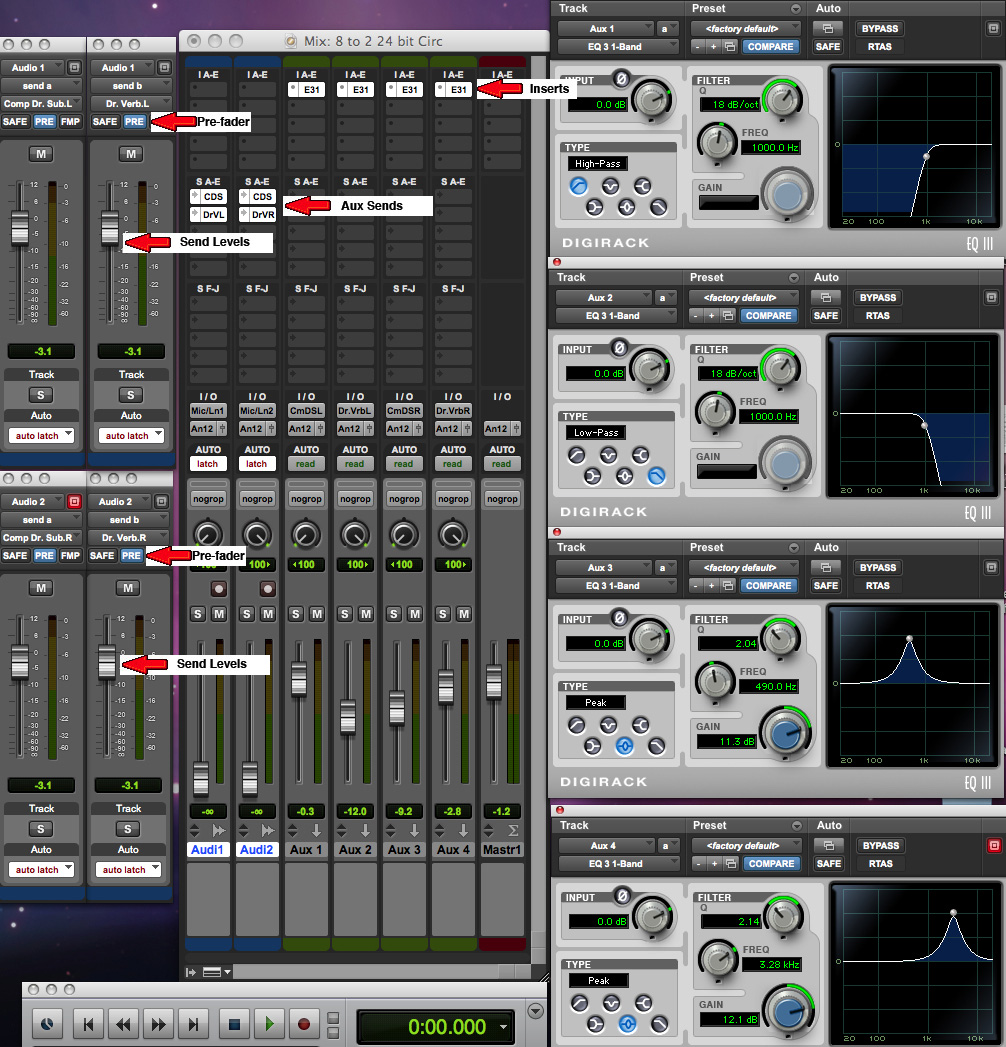
The diagram shows a
relatively simple parallel circuit in ProTools,
consisting of a stereo original track (of waves on a
shore), with four Auxiliary send buses selected
(at left) in “pre” mode to make them independent
of the original signal, with four Auxiliary returns
(in the middle) to mix the results with the original.
The four Auxiliary tracks have inserts that each
go to the simple 1-band filter/equalizer plug-in. These
have been chosen for high-pass, low-pass, a 1 kHz narrow
peak, and a 4 kHz narrow peak, respectively. The
Auxiliary returns are panned left and right in the mix.
The Master Gain is kept at -3 dB to avoid saturation. It
would be a good idea to save such a session as a template
for future use.
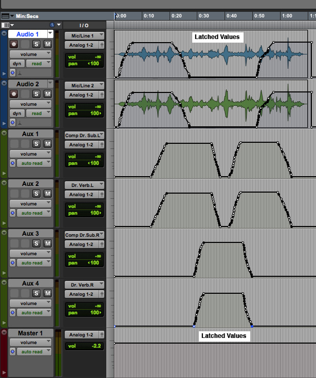
The 6 tracks are grouped into 3 stereo pairs to bring in
the original and the processed sounds together in stereo
pairs with similar level control. To keep the example
simple, all of the levels are shown in “latch”
mode which means that all level changes will be recorded
during the playback. The mouse control is therefore
limited to one of the three stereo sets of tracks at a
time, but a simple alternation between them can still be
effective.
(Click to
enlarge)
If you examine the above graphic of the
level controls, you’ll see the classic cross-fade
between each pair such that they overlap. Note that an
aurally effective cross-fade goes in three
stages: (1) bring in the first stereo track (2) bring
in the second stereo track to the desired level while
leaving the first track level intact (3) fade-out the
first track level, leaving the second one intact. This
pattern is repeated for all three combinations of
auxiliary signals, finally returning to the original.
All levels were controlled in a single playback.
This cross-fade pattern, which is a good aural
exercise requiring careful manual control if you want
to keep it smooth, is the opposite of what might be
implied by the symbol for cross-fade, namely X. A
literal X pattern, where the levels cross each other
in the middle, will leave a gap in loudness level
that is undesirable when a smooth result is wanted.
This example is quite subtle in terms of the changes
(the transition at 0:20 to the split high and low
filters, then at 0:40 to the narrow EQ pair, and then
returning by the same route to the original).
Something more dramatic could have been achieved by
using a multi-band processor so that the processed
sound was a combination of a narrow bandpass around
the levels that were being boosted, and therefore the
middle of the exercise would be just two narrow bands.
Waves processed with a parallel circuit (source: WSP
Can 41 take
2)
Of course, individual tracks can have
their levels individually controlled by soloing them
(or not) and latching only one set of stereo levels at
a time. However, that kind of track by track control
lacks some of the interaction that is desirable in a
parallel circuit. If you are fortunate enough to have
a digital mixing interface for the DAW, then
you can break free of the “tyranny of the mouse” which
only allows you to control one thing at a time. The
traditional mixer or its digital version capitalizes
on manual dexterity to control many levels at the same
time using your fingers, while guided by your ears.
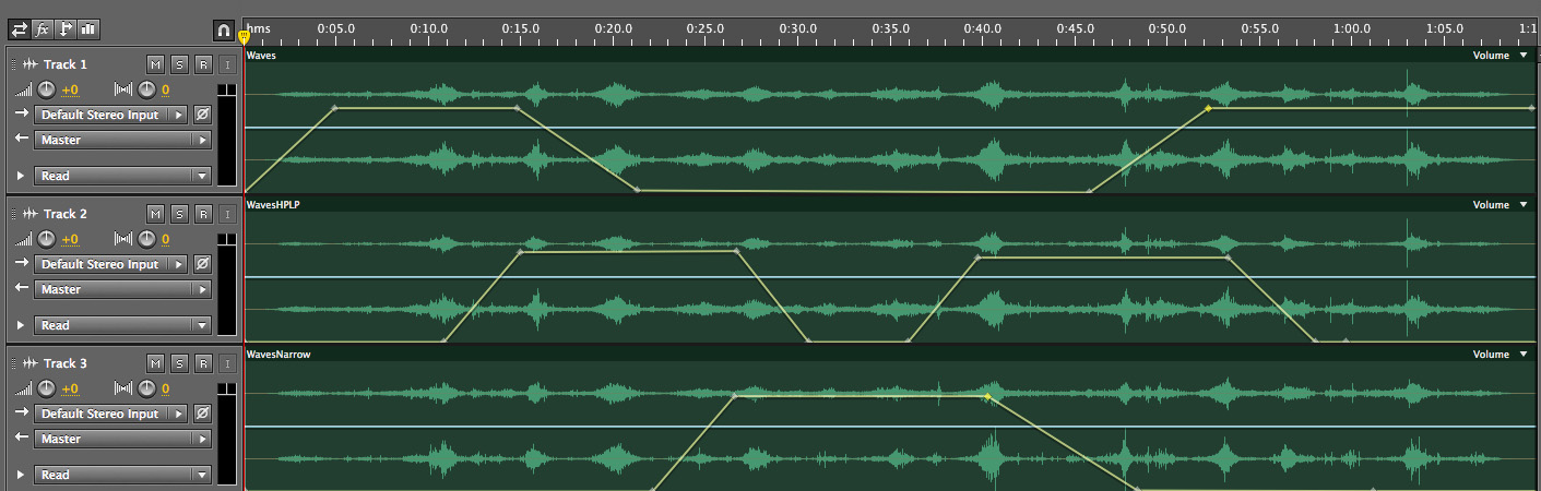
Parallel mixdown of the wave mix
Here is a similar result
achieved in a synchronous parallel
session in Audition. Again, there are three stereo
tracks, the original, the high-pass & low-pass
split spectrum, and a more dramatic narrow band
filtering with EQ boost, as mentioned above.
Audition simplified the process by allowing the
left and right channels to be modified separately
(by muting them one at a time when
applying the process to the unmuted channel) to
allow the higher and lower parts of the spectrum
to be distributed between the two channels for a
broader stereo effect. The session is
synchronous because each file starts at the
same time.
The session, shown graphically above, had its
levels determined by amplitude breakpoints
shown as yellow lines, with points of transition
determined by command clicks on the line, at which
time you see the specific dB level being chosen.
Since the waveform is silhouetted behind the
yellow line, it was simple to co-ordinate the peak
levels in each transition with a particular wave
(note the transitions at 0:26, 0:40 and 0:52).
Otherwise, classic cross-fades were followed.
d) Personal Studio Experiment No. 2
Based on the above examples, there are many
experiments that you could try out, using one or
more of the sounds you created in the first set of
experiments. Here are some suggestions:
1) Try setting up a parallel
session with a DAW that can be saved as a template
for future contexts. Experiment with a single
stereo sound source and get used to how the
various channel groupings and processor settings
are going to be controlled. Practice the classic
cross-fade when you start latching (i.e.
recording) level settings. If your DAW doesn’t
allow this, then use breakpoint amplitudes for
the same purpose. The main point of the
exercise, besides practicing the setup and
starting to feel comfortable with the Auxiliary
circuit, is to be able to create smooth, dynamic
mixes of variations of the same material.
2) If your editor incorporates multi-track
sessions as shown for Audition, try to duplicate
the DAW model in non-real-time. Otherwise, set
up a DAW multi-track session where you import
the already processed files. Notice how the
process differs and how the way you think about
it can evolve. Start with a synchronous version
just to keep things simple.
3) Try extending these processes to an asynchronous
session, using sounds that have been stretched
during the pitch transposition process from
Experiment 1. Start by lining up the files to
get an additive effect, being careful to control
the level of each so they are balanced but don’t
oversaturate. Shorter files can be copied one or
more times so they still sound while the longer
ones are progressing.
If your sound has a sharp attack, you may need
to shift the position of the lower pitched
versions because of the stretching. Usually this
can be done by zooming in on the files and
lining them up visually with a vertical cursor
line, then excising any extra silence. At the
end of each experiment, bounce the result to an
interleaved stereo file and check its
levels, etc. in an editor.


