![]()
Figure 2. Granular synthesis as a two-stage method.
Implementing Ecological Models
When developing ecological models, the emphasis is
not to obtain exact resynthesis of a given sound but to approximate the
behavior of a class of sounds. Thus, statistical descriptions and perceptually
relevant cues are more important than identical reproduction. In fact,
literal resynthesis of a sound which serves as a validity test for most
analysis / resynthesis techniques (Ellis, 1996; McAulay & Quartieri,
1986; Risset & Wessel, 1982), proves to be ecologically invalid. Ecological
models produce sounds that can be identified as belonging to the same class.
But each realization, or instance of given a model is never exactly the
same as any other instance of the same model.
Granular synthesis
More than a synthesis technique, "granular synthesis is a way of realizing sound production models using locally defined waveforms" (De Poli & Piccialli, 1991). Authors generally refer to any windowing technique as a form of granular synthesis. From a wide perspective, short-time Fourier transforms, wavelets, filterbanks, etc. would be included in granular synthesis methods (Cavaliere & Piccialli, 1997).
Looking at the granular approach as a two-stage method,
we can differentiate the control-function generation from the sound synthesis
stage. First, we establish a time-frequency grid of grains (Roads, 1996,
172) by means of analysis (Short-Time Fourier Transform, Wavelet Transform)
or algorithmic generation (screen, cloud, density). Then, we produce the
sound by placing either synthesized grains (e.g., sine waves, filter parameters)
or sampled-sound grains (from one or several sound files).
![]()
Figure 2. Granular synthesis as a two-stage method.
Table 3. Granular synthesis parameters.
|
|
|
|
|
|
|
|
|
|
|
|
|
|
|
|
|
|
|
|
Control functions
Whether the control functions are derived from analysis, or generated algorithmically, similarly to signals, they can be classified in two broad classes: (1) deterministic, and (2) stochastic. Paraphrasing Damper (1995, 258), a deterministic signal is one for which future values can be correctly predicted from a mathematical model of its generation process. Observed past values are used to find the parameters of the model. On the other hand, a stochastic signal is unpredictable because its generation process is too complex or poorly understood.
Deterministic processes can be produced by linear or nonlinear dynamical systems. A linear system is usually described by linear difference equations with constant coefficients (Damper, 1995, 36). Its output is a function of the input and the given coefficients (Bosch & Klauw, 1994, 9). These are some of the properties of linear systems: (a) the output is independent of previous inputs; (b) their impulse response is finite (FIR); (c) they are stable (Damper, 1995, 44). Examples of linear systems are the filters used in subtractive synthesis. By introducing feedback, the output of the system is made dependent on previous inputs. Thus, the impulse response becomes infinite and for some parameters the system may present instability and nonlinearity.
Based on these general classes of control functions, it is possible to group the synthesis methods in granular synthesis (as opposed to the analysis methods) in two rather simplified categories (Roads, 1997, 427): (1) synchronous, mostly based on deterministic functions; and (2) asynchronous, based on stochastic functions.
Synchronous methods are found in FOF synthesis (Rodet, 1984), VOSIM, quasi-synchronous GS, and pitch-synchronous granular synthesis (De Poli & Piccialli, 1991). Asynchronous methods have been used in synthesis by screens (Xenakis, 1971), real-time granular synthesis (Truax, 1988), FOG synthesis (Clarke, 1996), and pulsar synthesis (Roads, 1997). In this context, the functions control the delay between grains for a single stream. Alternately, Clarke (1996) measures the time between grain onsets and uses this parameter to control grain rate.
There are some limitations in the traditional control
method of independent grain streams, grain generators, or voices (Truax,
1988). As Clarke (1996) points out, these models do not take into account
the difference between synchronized and independent grain generators. In
ecologically-based granular synthesis, we use the term phase-synchronous
for several streams that share the same grain rate, and phase-asynchronous
for independent streams.
|
Synchronous stream |
Asynchronous stream |
|
Phase-synchronous streams |
Phase-asynchronous streams |
Figure 3. Classification of granular synthesis methods.
Sound database
As we mentioned previously, control functions define local parameters in granular synthesis. The relevance of each of these parameters depends on what GS approach is adopted. For example, envelope shape is important in FOF synthesis because this local parameter determines the bandwidth of the resulting formant. By contrast, the same parameter in asynchronous granular synthesis has little or no effect. Random sample-based processing causes spectral "blurring" and the sound is further modified by the complex interaction of overlapping spectrally rich grains. In part, this explains the gap between GS techniques that use simple synthetic grains to try to synthesize existing sounds, and the granular compositional approaches that start from more interesting and complex grains which produce less predictable results. "Tell me what grain waveform you choose and Ill tell you who you are."
A literature review has shown that GS techniques
have used three types of local waveforms: (1) sine waves, in FOF synthesis
(Rodet, 1984); (2) FIR filters derived by spectral analysis, in pitch-synchronous
synthesis (Cavaliere & Piccialli, 1997; De Poli & Piccialli, 1991);
and (3) arbitrary sampled sounds, in asynchronous granular synthesis (Truax,
1988), FOG (Clarke, 1996), and pulsar synthesis (Roads, 1997). Given that
the local spectrum affects the global sound structure, we have used grain
waveforms that can be parsed in short durations (20 to 200 ms) without
altering the complex characteristics of the original sampled sound. Thus,
we use water drops for stream-like sounds or pieces of bottles crashing
for breaking-glass sounds.
Methods
The synthesis technique used in our study is implemented in Csound (Vercoe, 1993), and the grain events are generated with our own score generator, CMask (Bartetzki, 1997), and Algorithmic Composer Toolbox (Berg, 1998). The local parameters provided by the score determine the temporal structure of the resulting sounds. These parameters are processed by one or several instruments in the orchestra. The instruments function as grain stream generators. There are three possible configurations: (1) a single stream generator, (2) parallel phase-asynchronous stream generators, (3) parallel phase-synchronous stream generators.
The total spectral result is given by the interaction
of the local waveforms with the meso-scale time patterns. Thus, the output
is characterized by emergent properties, which are not present in either
global or local parameters.
Table 4. Parameters of ecological models.
| Grain | Sound sample defined by: (1) frequency, (2) amplitude, (3) duration, (4) envelope shape, (5) sound file. |
| Grain pool | Several short sound files. Ecological models use complete sound events, i.e., the attack and decay of the recorded sounds are kept intact. Micro-models allow to apply transformations to the original samples. |
| Grain rate | Delay between the onset of two consecutive grains in the same stream. |
| Grain duration | Time interval between the onset and the end of the grain. |
| Grain amplitude | Maximum amplitude over grain duration. The control function is usually normalized to 1. |
| Grain frequency | Sample rate, expressed as a transposition ratio. 1 is the original sound file frequency. 2 raises an octave and cuts the duration of the sample to half its original length. |
| Grain sample | Spectral and micro-temporal content of the grain. It depends on the pointer location within the sound file. Several sound files can be used simultaneously. |
| Grain envelope | Shape of attack and decay of the grain. Quasi-Gaussian in asynchronous granular synthesis. Ecological models generally do not need windowing because they use pre-defined sample pools. |
| Grain overlap | Time interval during which two or more grains are sounding simultaneously. The grain overlap is determined by the difference between grain rate and grain duration. There are three possible configurations: (1) positive, there is a gap between the end of a grain and the onset of the following grain; (2) zero, a grain starts when the previous ends; (3) negative, before the grain ends the next one starts. There can be as many overlapping grains as memory and patience allow. |
| Stream | Grains synthesized by a single grain generator, i.e., one oscillator in the Csound orchestra. There are three implemented instruments (which can be extended): (1) single stream generator, (2) multiple phase-asynchronous stream generators, (3) multiple phase-synchronous stream generators. |
| File pointer | Location in sound file. These are the four possible ways to access the file contents: (1) no reset, the file is read from beginning to end; (2) loop, the file is read from beginning to end repeatedly; (3) cycle, the file is read from beginning to end and backwards repeatedly; (4) random, the file is read at randomly picked locations. The first one is the standard one. |
Procedure:
1. Collect several samples of everyday sounds produced by self-excited objects, such as running water or fire, and objects with an external source of energy, e.g., cracking wood, struck metal, etc.
2. Observe the temporal patterns and the spectral characteristics of the samples.
3. Extract grain samples to be used in the Csound synthesis language and define the meso-scale temporal behavior of the simulation.
4. Produce the synthetic sounds and compare results
with the original samples.
Bounce
The bounce pattern can be approximated by an exponential
curve or by a recursive equation. The former can only be used for one instance
of the class of bounce sounds. On the other hand, the latter provides a
general representation of all possible forms of bounce patterns. It can
easily be adjusted just by changing the damping parameter. This function
produces a family of exponential curves that we will use to control grain
rate and grain amplitude.
![]()
Figure 4. Bounce control function.
This function provides an idealized bounce pattern
in which damping is not affected by external factors such as surface irregularities
or shape of the bouncing object (assumed to be perfectly round). Furthermore,
we need to scale independently the damping factor controlling grain rate,
from the one controlling grain amplitude. We have found that the range
of damping values needs to be consistent with the objects elasticity.
When simulating bouncing bottles, the damping factor for grain amplitude
may be lower than the damping factor for grain rate. These settings allow
the grain rate to reach sub-audio rate before the amplitude has been completely
damped. The effect is a rising pitch that reproduces the phenomena heard
in real bouncing bottles.

Figure 5. Simple bounce model.
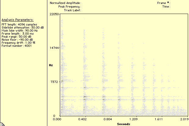
Figure 6. Spectrogram of bouncing bottles.
The initial grain rate is equivalent to the acoustic cue used to determine the distance between the bouncing object and the surface (in this context surface can also be understood as another object). Thus, if the first collision of object A occurs at 0 ms. and the second at 50 ms., and the first and second collisions of object B are at 0 ms. and 200 ms., we can safely infer that object B is initially more distant from the surface than A is, and that this difference is not determined by different elasticities. Contrastingly, the change over time in grain rate which is controlled by the damping factor provides a cue to the elasticity, or bounciness, of the object and the surface. Given the same surface, a very elastic object exhibits a slower acceleration in collision rate than a less bouncy one.
No surface is perfectly smooth and no object is perfectly
round. Therefore, random variations in bouncing behavior should be expected.
Given the inability of the auditory system to identify the source of these
random variations, i.e., is the surface uneven, or is the object not round?
We can express these irregularities as a single random parameter added
to the damping factor in the bounce function. The roughest surfaces and
the most irregular objects get the highest random variations. Similarly,
a pool of varied grain samples can be used to account for changes in spectral
characteristics at a micro level. Therefore, a more refined bounce model
should include random changes in grain rate, grain amplitude, and grain
sample. Time-dependent changes in spectral profile, to account for progressive
loss of energy, could also be included.
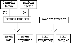
Figure 7. A more refined bounce model.
No sound in nature happens exactly the same way twice. The unnatural quality of loops and repeated sample playback is caused by the lack of variation at the micro and meso-level sound organization. The auditory system can readily recognize sounds with micro-level repetitions as ecologically unfeasible events (Tróccoli & Keller, 1996). On the other hand, sudden changes in micro-level characteristics usually cue the beginning of a new event. Thus, synthesized environmental sounds should exhibit dynamic micro-level characteristics within carefully constrained ranges.
In models that use sampled grains, grain frequency
stands for change in sample rate. This rate is expressed as a ratio. Thus,
1.0 keeps the original sample rate and 0.5 drops the frequency one octave
and doubles the length of the sampled sound. We have observed that variations
in a range of 0.1% (.001) to 10% (.1) produce very subtle to dramatic effects.
Of course, this depends on the interaction with other variables and on
the characteristics of the samples used.
Scrape
The scrape model that will be discussed in this section is based on the assumption of a single point / surface interaction. This is clearly an idealized case but provides a basis for more complex models that could be controlled by high-level transformations. The results obtained with this model are perceptually more satisfying than the ones reported in (Gaver, 1993, 233), i.e., frequency of band-limited noise corresponding to dragging speed, and filter bandwidth correlated to roughness of the surface.
Scraping is usually linked to gestures produced by human agents. Therefore, scrape events should be constrained to finite durations feasible by human movement (unless the acoustic cues are intended to suggest a machine-generated process). The ecological event satisfies perfectly these requirements. Given this context, the scraping action cannot start suddenly from a high-energy level but needs to develop slowly from zero amplitude. To mimic this behavior, we use a tendency mask which allows for random variations in grain amplitude and constrains the initial and final ranges to zero. Similarly, increase or decrease in scrape speed happens at relatively slow rates. We simulate scraping action by controlling the grain rate with a fairly simple algorithm.
The scrape function consists of a random number generator
that sends values uniformly distributed over zero and under zero to an
accumulator. The requirement of a single absolute limit for positive and
negative values is needed to avoid overflowing the accumulator or getting
stuck at a boundary value. The accumulator is limited by a low and a high
boundary which establishes the fastest and slowest possible rates. Depending
on the number of positive or negative values produced by the number generator,
the scraping speed increases or decreases accordingly. The absolute limit
value given to the number generator defines a virtual time grid, grid
factor. If this value is high the delay among grains is usually long,
if it is slow average grain rate will be fast.
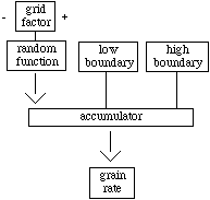
Figure 8. Scrape control function.
Aside from the gestural action produced by a human
agent, scraping is also determined by the characteristics of the surface
being scraped. Given that the gesture is assumed to be fairly constant,
irregularities in the rate of interaction between point and surface can
be attributed to surface roughness. By randomizing the grain rate control
by a small percentage (up to 10%), we obtain various degrees of roughness
without affecting the gestural feel of the model. The material of the surface
being scraped is established by the timbral quality of recorded grains
or by modifying the spectral result through the use of resonators.
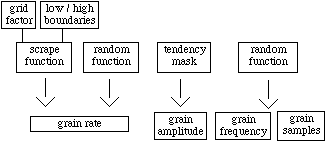
Figure 9. Simple scrape model.
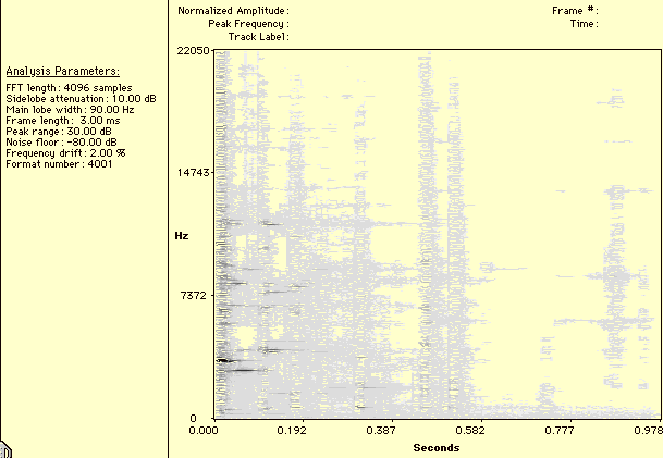
Figure 10. Spectrogram of breaking glass.
Break
Breaking patterns are time-varying, highly structured events. Straightforward random distributions or superimposed bounce patterns (Warren & Verbrugge, 1984) do not approximate the complex behavior of these sounds. A multi-level approach is needed. Careful observation of recorded breaking glass sounds provides some useful insights. The initial strike produces broadband resonances in the whole object. These resonances last for approximately five milliseconds and can be simulated with an enveloped burst of white noise. As explained in (Keller & Rolfe, 1998), the envelope shape provides a simple way to filter out high frequencies. Alternatively, a sampled grain can be used.
After the first five to ten milliseconds the object starts to break. Many small pieces hit a surface (possibly the floor) producing a dense cloud of impacts. Although these sounds share the spectral characteristics of the whole object, given the pieces small size their spectral profile has a higher frequency content. A more noisy sound is produced by glass pieces hitting each other. Thus, it seems reasonable to use a short-impact grain pool with two spectral characteristics: glass hitting a surface, and glass hitting glass. The amplitude of these impacts can be approximated by an exponential decay.
A third complex sub-event in breaking consists of
randomly varying bouncing patterns. These patterns are produced by pieces
scattered around the initial impact spot. Depending on the surface elasticity
and the shape of the broken pieces, these patterns range from highly random
with high damping factor to slightly random with low damping factor. The
last configuration produces bounce-like patterns. The algorithms used for
bouncing can be used to produce these meso patterns.

Figure 11. Breaking glass model.
Summarizing, breaking glass is composed of three
sub-events: (1) A broadband attack, lasting five to ten milliseconds. (2)
A dense random cloud of short impacts: glass onto surface and glass onto
glass, lasting less than fifty milliseconds. (3) Several overlapped bouncing
patterns with durations depending on the surface elasticity (one second
or more).
Summary
This section discussed the implementation details
of ecological models, focusing on three examples: bouncing, scraping, breaking.
Ecological models use grain pools of isolated meaningful events taken from
real-world sounds. The distribution of grains is controlled from meso-level
functions, following patterns found in nature.
|
|
|
|
|
|
|
|
|