STAT 350: Lecture 23

Goodness-of-fit: Pure Error Sum of Squares, An Example

• Plaster hardness data of Lecture 12.
• 9 different covariate patterns: 3 levels of SAND and 3 levels of FIBRE.
• Two ways to compute pure error sum of squares:
  • Create new variable with 9 levels.
  • Fit a two way ANOVA with interactions.

DATA

0 0 1 61 34

0 0 1 63 16

15 0 2 67 36

15 0 2 69 19

30 50 9 74 48

SAS CODE

  data plaster;
  infile 'plaster1.dat';
  input sand fibre combin hardness strength;
  proc glm  data=plaster;
   model hardness = sand fibre;
  run;
  proc glm  data=plaster;
   class sand fibre;
   model hardness = sand | fibre ;
  run;
  proc glm  data=plaster;
   class combin;
   model hardness = combin;
  run;

EDITED OUTPUT

                            Sum of          Mean
Source DF        Squares        Square  F Value  Pr > F
Model   2   167.41666667   83.70833333   11.53   0.0009
Error  15   108.86111111    7.25740741
Total  17   276.27777778
_______________________________________________________
                            Sum of          Mean
Source DF        Squares        Square  F Value  Pr > F
Model   8   202.77777778   25.34722222     3.10  0.0557
Error   9    73.50000000    8.16666667
Total  17   276.27777777
_______________________________________________________
                           Sum of          Mean
Source DF        Squares        Square  F Value  Pr > F
Model   8   202.77777778   25.34722222    3.10   0.0557
Error   9    73.50000000    8.16666667
Total  17   276.27777778

From the output we can put together a summary ANOVA table

Source df SS MS F P

Model 2 167.417 83.708

Lack of Fit 6 35.361 5.894 0.722 0.64

Pure Error 9 73.500 8.167

Total (Corrected) 17 276.278

• The F statistic is [( 108.86111111 - 73.50000000)/6]/[8.16666667].
• The P-value comes from the distribution.
• The P-value is not significant so there is no reason to reject the final fitted model which was additive and linear in each of SAND and FIBRE.
• Notice that the Error SS are the same for the two-way ANOVA with interactions, which is the second model, and for the 1 way ANOVA.
• This test is not very powerful in general; more sensitive tests are available if you know how the model might break down. For instance, most realistic alternatives will be picked up more easily by checking for quadratic terms in a bivariate polynomial model as done in class in Lecture 11.
• Notice that the test for any effect of SAND and FIBRE carried out in the one way analysis of variance is not significant. This is an example of the lack of power found in many F-tests with large numbers of degrees of freedom in the numerator. If you can guess a reasonable functional form for the effect of the factors (either the additive two way model with no interactions or the even simpler multiple regression model which is the first model above) you will get a more sensitive test usually.

Making an Added variable plot: example

• For SCENIC data to assess influence of facilities.
• Regress RISK on STAY, CULTURE, NURSES, NURSE.RATIO. Get residuals.
• Regress FACILITIES on STAY, CULTURE, NURSES, NURSE.RATIO. Get residuals.
• Plot residuals against each other. Look for patterns.

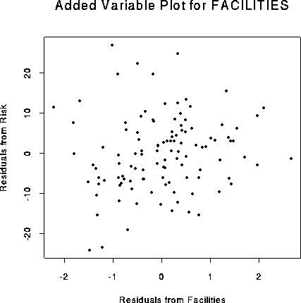
Here is the added variable plot:

Categorical Covariates

• Examples: variables SCHOOL (Med school yes or no) and REGION.
• Called Factors, possible values called levels; e.g. YES or NO are 2 levels of factor SCHOOL.
• Simplest situation when effects additive: intercepts depend on levels of categorical covariates but not slopes of other variables. Idea is: effect of NURSES is measured by corresponding slope. Interpretation simplest if slope same for schools in all 4 regions.
• See assignment 3 for simplest example.
• If slope depends on level of categorical covariate then factor interacts with continuous covariate, otherwise effects called additive.

Fitting models with categorical covariates

Suppose a categorical variable has K levels. Relabel the data as where j runs from 1 to and i runs from 1 to K. Here is the number of observations with the categorical variable at level i. We fit the model

where now is the vector of slopes for, say, p continuous covariates and is the intercept which depends on the level i of the categorical variable.

This model does not have a column of 1's in the design matrix. It can be fitted by specifying /NOINT in SAS, for example. It is common, however, to reparametrize in such a way that the model has a column of 1's and the hypothesis of no effect of the factor, that is, is simply the hypothesis that the coefficients of some columns of the design matrix are 0. We usually do this by defining to be a weighted average of the intercepts, that is,

or by defining to be the intercept for level 1 of the factor, that is, . In either case we define some new parameters . The model equation is now

Notice that in either case the satisfy a linear restriction: either

or

If we forget about this linear restriction then our linear reparametrization increases the number of columns of the design matrix by 1 but without increasing the rank of X so that the new would be singular. SAS does the algebra without worrying about this by simply finding 1 of infinitely many possible solutions to the normal equations. I usually suggest the definition of as an average intercept. Then I eliminate by writing

This changes the rows of the design matrix corresponding to observations at level K. The other definition of as is called corner point coding and the column of the design matrix corresponding to is dropped.

Example

Consider a small version of the car mileage example on assignment 3. Imagine we have only the 5 data points below.

VEHICLE 1 VEHICLE 2

Mileage Emission Rate Mileage Emission Rate

0 50 0 40

1000 56 1100 49

2000 58

For the model equation

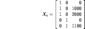
we have , . The are the 5 numbers 0, 1000, 2000, 0, 1100. For this parametrization the design matrix is

For the parametrization

the design matrix simply is that above with an extra colmn of 1's:

Since columns 2 and 3 add together to give the first column the matrix has rank 4 and is singular.

If we define the parameters , and then . As a result we can write the model equations as

and

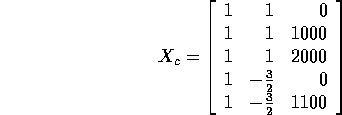
and then the design matrix is

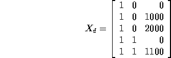
Alternatively corner point coding leads to the design matrix

All these design matrixes have the same column spaces so they must lead to the same fitted values, same residuals and the same error sum of squares. The hypothesis of no "Vehicle" effect, that is, that the two cars have the same intercept is tested either by a t-test on the parameter which is the difference of intercepts or by an extra sum of squares F-test comparing with the restricted model in which just 1 straight line is fitted.

One important point is that in all the parametrizations the parameter "difference of intercepts" has the same estimate. This is true even for the matrix for which is singular.

Factors with more than two levels

Let us now examine what happens if we add two categorical variables, SCHOOL and REGION, to our model using sas.

SAS CODE

options pagesize=60 linesize=80;
data scenic;
 infile 'scenic.dat' firstobs=2;
 input Stay  Age Risk Culture Chest Beds 
       School Region Census Nurses Facil;
 Nratio = Nurses / Census  ;
proc glm  data=scenic;
  class School Region;
  model Risk = Culture Stay Nurses 
     Nratio School Region;
run ;
proc glm  data=scenic;
  class School Region;
  model Risk = Culture Stay 
    Nurses School Region;
run ;
proc glm  data=scenic;
  class School Region;
  model Risk = Culture Stay Nurses Region;
run ;

EDITED OUTPUT

                           Class    Levels    Values
                           SCHOOL        2    1 2
                           REGION        4    1 2 3 4
Dependent Variable: RISK   
                     Sum of            Mean
Source     DF       Squares          Square   F Value     Pr > F
Model       8  110.94402256     13.86800282     15.95     0.0001
Error     104   90.43580045      0.86957500
Total     112  201.37982301
     R-Square      C.V.        Root MSE            RISK Mean
     0.550919   21.41305       0.9325101            4.3548673
Source     DF     Type I SS     Mean Square   F Value     Pr > F
CULTURE     1   62.96314170     62.96314170     72.41     0.0001
STAY        1   27.73884588     27.73884588     31.90     0.0001
NURSES      1    7.01369438      7.01369438      8.07     0.0054
NRATIO      1    5.97484076      5.97484076      6.87     0.0101
SCHOOL      1    1.24877748      1.24877748      1.44     0.2335
REGION      3    6.00472236      2.00157412      2.30     0.0815
Source     DF   Type III SS     Mean Square   F Value     Pr > F
CULTURE     1   27.43863928     27.43863928     31.55     0.0001
STAY        1   26.44898274     26.44898274     30.42     0.0001
NURSES      1    6.39021516      6.39021516      7.35     0.0079
NRATIO      1    1.74482880      1.74482880      2.01     0.1596
SCHOOL      1    2.21945688      2.21945688      2.55     0.1132
REGION      3    6.00472236      2.00157412      2.30     0.0815
________________________________________________________________
                     Sum of            Mean
Source     DF       Squares          Square   F Value     Pr > F
Model       7  109.19919376     15.59988482     17.77     0.0001
Error     105   92.18062925      0.87791075
Total     112  201.37982301
     R-Square      C.V.        Root MSE            RISK Mean
     0.542255   21.51544       0.9369689            4.3548673
Source     DF     Type I SS     Mean Square   F Value     Pr > F
CULTURE     1   62.96314170     62.96314170     71.72     0.0001
STAY        1   27.73884588     27.73884588     31.60     0.0001
NURSES      1    7.01369438      7.01369438      7.99     0.0056
SCHOOL      1    2.16544259      2.16544259      2.47     0.1193
REGION      3    9.31806922      3.10602307      3.54     0.0173
Source     DF   Type III SS     Mean Square   F Value     Pr > F
CULTURE     1   32.63679640     32.63679640     37.18     0.0001
STAY        1   24.70628794     24.70628794     28.14     0.0001
NURSES      1    8.99075614      8.99075614     10.24     0.0018
SCHOOL      1    3.19583271      3.19583271      3.64     0.0591
REGION      3    9.31806922      3.10602307      3.54     0.0173
________________________________________________________________
                     Sum of            Mean
Source     DF       Squares          Square   F Value     Pr > F
Model       6  106.00336105     17.66722684     19.64     0.0001
Error     106   95.37646196      0.89977794
Corrected Total     112     201.37982301
        R-Square    C.V.        Root MSE            RISK Mean
       .526385   21.78175       0.9485663            4.3548673
Source     DF     Type I SS     Mean Square   F Value     Pr > F
CULTURE     1   62.96314170     62.96314170     69.98     0.0001
STAY        1   27.73884588     27.73884588     30.83     0.0001
NURSES      1    7.01369438      7.01369438      7.79     0.0062
REGION      3    8.28767910      2.76255970      3.07     0.0310
Source     DF   Type III SS     Mean Square   F Value     Pr > F
CULTURE     1   30.50324858     30.50324858     33.90     0.0001
STAY        1   22.98974524     22.98974524     25.55     0.0001
NURSES      1    5.85040582      5.85040582      6.50     0.0122
REGION      3    8.28767910      2.76255970      3.07     0.0310

CONCLUSIONS

• Look at type III SS to see which effects can be deleted from full model. BUT, can only delete one at a time. Notice that NRATIO is least significant so drop it and refit.
• After refitting SCHOOL is not quite significant so delete and rerun. All remaining effects significant.
• Notice that F-test for REGION has 3 degrees of freedom. What is being tested is where these are 4 intercepts. Under the restricted model where this hypothesis is assumed there is 1 intercept compared to 4 intercepts in the full model. The difference of 3 is the degrees of freedom associated with the sum of squares for REGION.
• The TYPE III sums of squares are extra SS for comparing a model with all the effects in the model statement in proc glm to a model with one of those effects removed (but all the others still there).
• The TYPE I SS are also called sequential SS. They compare models which include all the factors down to a certain line in the table with the model including all the factors down to that line but not including the line. So, for example, the Type I SS for SCHOOL in the first model compares a model with CULTURE, STAY, NURSES and NRATIO to a model with all those variables plus SCHOOL. Neither model includes the line lower than SCHOOL in the table, that is, neither model includes REGION. All the TYPE I F-statistics use the ESS from the whole model fitted by GLM in the denominator (so the denominator estimate of in Type I SS test for Schools is the ESS from a model including REGION as well as all the other variables.