STAT 350: Lecture 35

Estimating equations: an introduction via glm

Estimating Equations: refers to equations of the form

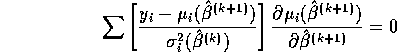
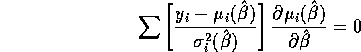
which are solved for to get estimates . Examples:

1. The normal equations in linear regression:

   

2. The likelihood equations:

   

   where is the log-likelihood.

3. The equation which must be solved to do non-linear least squares:

   

4. The iteratively reweighted least squares estimating equation:

   

   where, in a generalized linear model the variance is a known (except possibly for a multiplicative constant) function of .

Only the first of these equations can usually be solved analytically. In Lecture 34 I showed you an example of an iterative technique of solving such equations.

Theory of Generalized Linear Models

The likelihood function for a Poisson regression model is:

and the log-likelihood is

A typical glm model is

where the are covariate values for the ith observation (often including an intercept term just as in standard linear regression).

In this case the log-likelihood is

which should be treated as a function of and maximized.

The derivative of this log-likelihood with respect to is

If has p components then setting these p derivatives equal to 0 gives the likelihood equations.

For a Poisson model the variance is given by

so the likelihood equations can be written as

which is the fourth equation above.

These equations are solved iteratively, as in non-linear regression, but with the iteration now involving weighted least squares. The resulting scheme is called iteratively reweighted least squares.

1. Begin with a guess for the standard deviations (taking them all equal to 1 is simple).
2. Do (non-linear) weighted least squares using the guessed weights. Get estimated regression parameters .
3. Use these to compute estimated variances . Go back to do weighted least squares with these weights and get .
4. Iterate (repeat over and over) until estimates not really changing.

If the converge as to something, say, then since

we learn that must be a root of the equation

which is the last of our example estimating equations.

Distribution of Estimators

Distribution Theory is the subject of computing the distribution of statistics, estimators and pivots. Examples in this course are the Multivariate Normal Distribution, the theorems about the chi-squared distribution of quadratic forms, the theorems that F statistics have F distributions when the null hypothesis is true, the theorems that show a t pivot has a t distribution.

Exact Distribution Theory: name applied to exact results such as those in previous example when the errors are assumed to have exactly normal distributions.

Asymptotic or Large Sample Distribution Theory: same sort of conclusions but only approximately true and assuming n is large. Theorems of the form:

• An estimate is normally only useful if it is equipped with a measure of uncertainty such as a standard error.
• A standard error is a useful measure of uncertainty provided the error of estimation has approximately a normal distribution and the standard error is the standard deviation of this normal distribution.
• For many estimating equations the root is unique and has the desired approximate normal distribution, provided the sample size n is large.

Sketch of reasoning in special case

POISSON EXAMPLE: p=1

Assume has a Poisson distribution with mean where now is a scalar.

The estimating equation (the likelihood equation) is

It is now important to distinguish between a value of which we are trying out in the estimating equation and the true value of which I will call . If we happen to try out the true value of in U then we find

On the other hand if we try out a value of other than the correct one we find

But is a sum of independent random variables so by the law of large numbers (law of averages) must be close to its expected value. This means: if we stick in a value of far from the right value we will not get 0 while if we stick in a value of close to the right answer we will get something close to 0. This can sometimes be turned in to the assertion:

The glm estimate of is consistent, that is, it converges to the correct answer as the sample size goes to .

The next theoretical step is another linearization. If is the root of the equation, that is, , then

This is a Taylor's expansion. In our case the derivative is

so that approximately

The right hand side of this formula has expected value 0, variance

which simplifies to

This means that an approximate standard error of is

that an estimated approximate standard error is

Finally, since the formula shows that is a sum of independent terms the central limit theorem suggests that has an approximate normal distribution and that

is an approximate pivot with approximately a N(0,1) distribution. You should be able to turn this assertion into a 95% (approximate) confidence interval for .

Scope of these ideas

The ideas in the above calculation can be used in many contexts.

• We can get approximate standard errors in non-linear regression.
• We can get approximate standard errors in any model where we do maximum likelihood.
• We can show that the assumption of normal errors does not have too big an impact on the t and F tests in multiple regression.
• We can get approximate standard errors in generalized linear models.
• We can demonstrate that the role of the Error Sum of Squares in multiple regression can be replaced, approximately, by a function called the Deviance which is a function whose derivative (with respect to the parameters) is the estimating equation.

Further exploration of the ideas in this course

• STAT 402 explores applications of generalized models.
• STAT 410 applies regression to samples from finite populations.
• STAT 420 discusses the analysis of variance and regression when the normality assumption seems very probably wrong.
• STAT 430 discusses the design and analysis of experiments. Topics include: designs which save on effort by deliberately making singular, the advantages of randomized controlled experiments, justification of t and F tests by randomization rather than sampling arguments, experiments in which (some of) the s are random.
• STAT 450 discusses the exact and approximate distribution theory discussed here, along with mathematical justifications for using tests and estimates recommended here and in other courses as opposed to any others.
• STAT 802 explores problems in which each is multivariate, that is, there is more than 1 response variable.
• STAT 804 (Time Series Analysis) explores problems in which the errors are not independent.