No Title

$next$ $up$ $previous$

STAT 350: Lecture 34

Non-linear Regression

In a regression model of the form

we call the model linear if for some covariates and a parameter . Often, however, we have non-linear models such as or in general for some function f which need not be linear in . If the errors are homo-scedastic normal errors then the maximum likelihood estimates of the are least squares estimates, minimizing . The value then solves

This equation can usually not be solved analytically. In general the process of solving it numerically is iterative. One approach is:

Begin with an initial guess (no general method available to do this step) for the parameter estimates, say .
Linearize the function around by doing a Taylor expansion. This involves writing

where is the vector of partial derivatives of with respect to the entries in .
Replace in the sum of squares by this approximation and get that you are trying to minimize

with respect to .
This is really now an ordinary least squares problem in which we are regressing on . Let be the matrix with ith row where the derivative is evaluated at . Then we are to minimize

where . The solution is . We compute this .
Update to .
Recompute the entries in X with the new value , get a new then a and so on.
Continue until the estimates change little or the sum of squares changes little.

Example

In thermoluminescence dating ( see Lecture 1) a common model is

Thus in this case

The derivatives of with respect to the entries of are

and

Software and computing details

In SAS the procedure proc nlin will do non-linear least squares. You need to specify quite a few ingredients. The model statement must specify the exact functional form of the function . You have a statement parms which is needed to specify the initial guess for . You usually will have a bunch of der statements to specify derivatives of the predicted values with respect to each parameter and, if you use some algorithms, you will even specify some second derivatives. (You get a choice of 5 different iterative algorithms. The one described above is called Gauss-Newton.)

In Splus the function nls can be used to to the same thing.

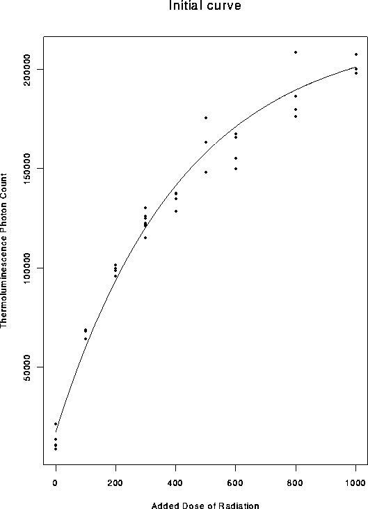
Here is a plot of some thermoluminescence data.

Superimposed on the picture is the curve above for the values

and

I will analyze the data by using the Gauss-Newton algorithm by hand and then using glm and nlin

S-PLUS : Copyright (c) 1988, 1996 MathSoft, Inc.
S : Copyright AT&T.
Version 3.4 Release 1 for Sun SPARC, SunOS 5.3 : 1996 
Working data will be in .Data 
> > dat <- read.table("satur.data",header=T)
> #
> #  Read in data
> #
> beta0 <- 220000
> #
> #  From looking at picture guess saturation level
> #
> beta <- lsfit(dat$Dose,-log(1-dat$Count/beta0))$coef
> #
> #  Get initial values for beta by solving
> #   y = b1(1-exp(-(x-b2)/b3)) to get
> #   log(1-y/b1) = -(x-b2)/b3 and then regressing
> #   log(1-y/b1) on dose.
> #
> beta <- lsfit(dat$Dose,-log(1-dat$Count/beta0))$coef
> beta[2] <- 1/beta[2]
> beta[1] <- -beta[2]*beta[1]
> beta <- c(beta0,beta)
> beta
        Intercept        X 
 220000 -34.46809 422.0629
> #
> #  These are the initial estimates
> #
> dv <- seq(0,max(dat$Dose),length=300)
> cv <- beta[1]*(1-exp(-(dv-beta[2])/beta[3]))
> postscript("curve0.ps",horizontal=F)
> plot(dat$Dose, dat$Count,xlab="Added Dose of Radiation",
+    ylab="Thermoluminescence Photon Count",main="Initial curve")
> lines(dv,cv)
> dev.off()
Generated postscript file "curve0.ps".
 null device 
           1
> #
> #   Plot the initial curve on top of the data.
> #
> fder <- function(d,b){
+ #
+ # This function computes derivatives of 
+ #  mu with respect to each component of 
+ #  beta and assembles them into a matrix
+ #
+     v <- exp(-(d-b[2])/b[3])
+     cbind(1-v,-v*b[1]/b[3],-b[1]*(d-b[2])*v/b[3]^2)
+ }
> mu_function(d,b){
+ #
+ # This function computes the vector mu
+ #  of fitted values 
+ #
+    b[1]*(1-exp(-(d-b[2])/b[3]))
+ }
> #
> #   Plot the initial curveon top of the data.
> #
> postscript("curves.ps",horizontal=F)
> plot(dat$Dose, dat$Count,xlab="Added Dose of Radiation",
+    ylab="Thermoluminescence Photon Count",main="Initial curve")
> lines(dv,cv)
> #
> #  Here we regress the original Ys minus the current fit on the
> #  derivative of the fit with respect to the parameters.
> #
> ystar <- dat$Count -mu(dat$Dose,beta)
> delta <- lsfit(fder(dat$Dose,beta),ystar,intercept=F)$coef
> beta1 <- beta+delta
> beta <- beta1
> print(delta)
        X1        X2        X3 
 -9433.193 0.8641427 -33.86906
> #
> #   The increment in the fitted beta vector
> #
> cv <- beta[1]*(1-exp(-(dv-beta[2])/beta[3]))
> lines(dv,cv,lty=2)
> #
> #   Add a curve to the plot for the new beta vector
> #    and then repeat the process
> #
> ystar <- dat$Count -mu(dat$Dose,beta)
> delta <- lsfit( fder(dat$Dose,beta),ystar,intercept=F)$coef
> beta2 <- beta+delta
> print(delta)
        X1        X2        X3 
 -115.2705 0.5834134 -1.532228
> beta <- beta2
> cv <- beta[1]*(1-exp(-(dv-beta[2])/beta[3]))
> lines(dv,cv,lty=3)
> #
> #   Add a curve to the plot for the new beta vector
> #    and then repeat the process
> #
> ystar <- dat$Count -mu(dat$Dose,beta)
> delta <- lsfit( fder(dat$Dose,beta),ystar,intercept=F)$coef
> beta3 <- beta+delta
> print(delta)
        X1         X2         X3 
 -26.40946 0.02285527 -0.1350775
> beta <- beta3
> cv <- beta[1]*(1-exp(-(dv-beta[2])/beta[3]))
> lines(dv,cv,lty=4)
> #
> #   Add a curve to the plot for the new beta vector
> #    and then repeat the process
> #
> ystar <- dat$Count -mu(dat$Dose,beta)
> delta <- lsfit( fder(dat$Dose,beta),ystar,intercept=F)$coef
> beta4 <- beta+delta
> print(delta)
        X1          X2          X3 
 -2.416176 0.002208632 -0.01256684
> beta <- beta4
> cv <- beta[1]*(1-exp(-(dv-beta[2])/beta[3]))
> lines(dv,cv,lty=5)
> #
> #   Add a curve to the plot for the new beta vector
> #    and then repeat the process
> #
#                    Intercept           X 
# beta0 220000.0     -34.46809    422.0629
# beta1 210566.8     -33.60395    388.1938
# beta2 210451.5     -33.02054    386.6616
# beta3 210425.1     -32.99768    386.5265
# beta4 210422.7     -32.99547    386.5139
> dev.off()
Generated postscript file "curves.ps".
 null device 
           1
> q() # end-of-file

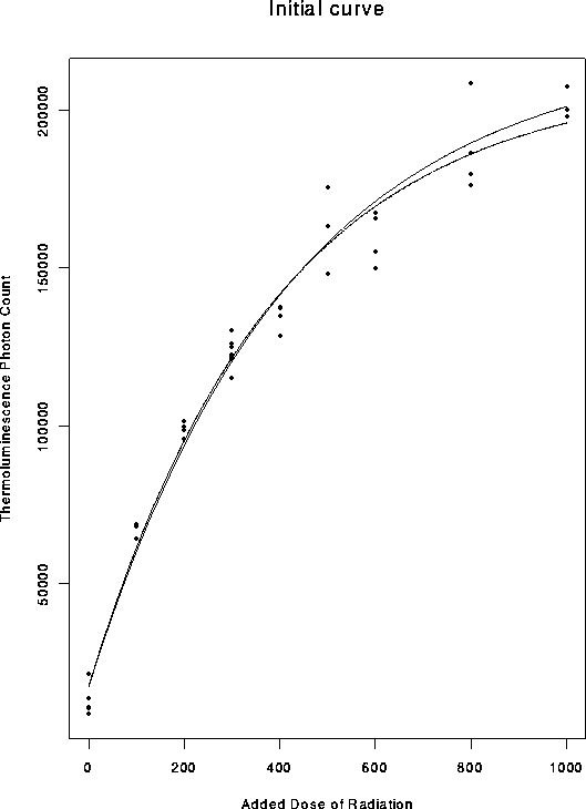
The successive fits are plotted here:

Here is SAS code for the same problem

options pagesize=60 linesize=80;
data thermo;
 infile 'satur.data' firstobs=2;
 input Code Dose Count ;
proc nlin  data=thermo;
 parms b1=220000  b2=-34.46809 b3=422.0629;
 model Count = b1*(1-exp(-(Dose - b2)/b3));
 der.b1=(1-exp(-(Dose - b2)/b3));
 der.b2=-b1*exp(-(Dose - b2)/b3)/b3;
 der.b3=-b1*(Dose - b2)*exp(-(Dose - b2)/b3)/b3**2;
run;

producing the output

                    Non-Linear Least Squares Iterative Phase
                Dependent Variable COUNT   Method: Gauss-Newton
       Iter       B1             B2             B3       Sum of Squares
          0         220000     -34.468090     422.062900     2824928590
          1         210567     -33.603952     388.193816     2670087246
          2         210452     -33.020538     386.661589     2669527014
          3         210425     -32.997683     386.526512     2669525464
          4         210423     -32.995474     386.513945     2669525451
NOTE: Convergence criterion met.
    Non-Linear Least Squares Summary Statistics     Dependent Variable COUNT
        Source                DF Sum of Squares     Mean Square
        Regression             3   679415907744    226471969248
        Residual              35     2669525451        76272156
        Uncorrected Total     38   682085433194
        (Corrected Total)     37   122311153163
        Parameter     Estimate    Asymptotic             Asymptotic 95 %
                                  Std. Error         Confidence Interval
                                                     Lower         Upper
        B1         210422.7105  6587.3455230  197049.76755  223795.65354
        B2            -32.9955     8.2899354     -49.82484     -16.16611
        B3            386.5139    31.3425426     322.88558     450.14231
                         Asymptotic Correlation Matrix
           Corr                B1                B2                B3
           ----------------------------------------------------------
           B1                   1      -0.442969052      0.9150075187
           B2        -0.442969052                 1      -0.663625494
           B3        0.9150075187      -0.663625494                 1

$next$ $up$ $previous$

Richard Lockhart
Tue Mar 25 11:02:59 PST 1997