NOTE: This material may be covered later in the course. The next section of the course is labelled Inference.
STAT 270 version of central limit theorem:
if
![]() are iid from a population with mean
are iid from a population with mean ![]() and standard
deviation
and standard
deviation ![]() then
then
![]() has approximately
a normal distribution.
has approximately
a normal distribution.
Also Binomial![]() random variable
has approximately a
random variable
has approximately a
![]() distribution.
distribution.
Precise meaning of statements
like ``![]() and
and ![]() have approximately the same distribution''?
have approximately the same distribution''?
Desired meaning: ![]() and
and ![]() have nearly the same cdf.
have nearly the same cdf.
But care needed.
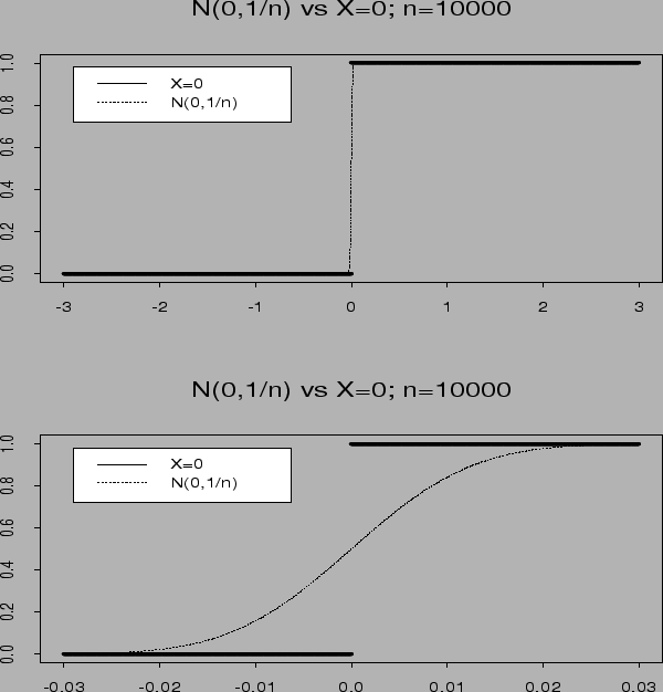
Q1) If ![]() is a large number is the
is a large number is the
![]() distribution close to the distribution of
distribution close to the distribution of ![]() ?
?
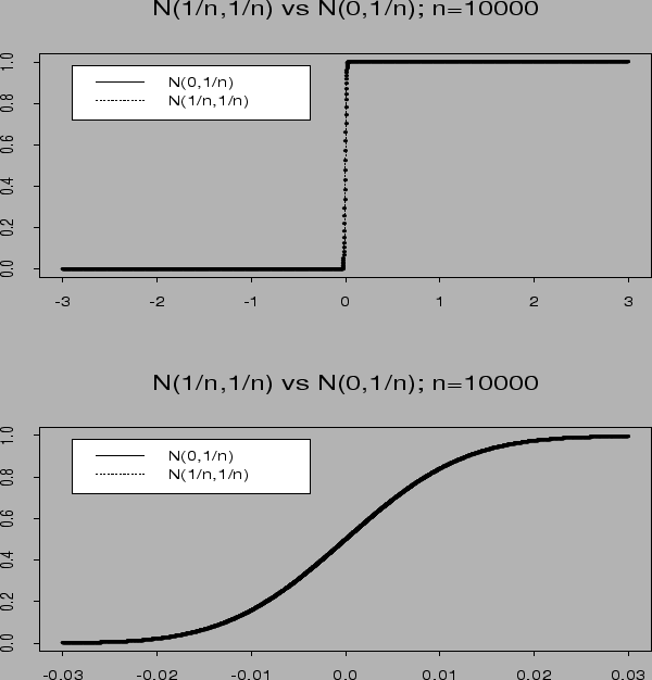
Q2) Is ![]() close to the
close to the
![]() distribution?
distribution?
Q3) Is ![]() close to
close to
![]() distribution?
distribution?
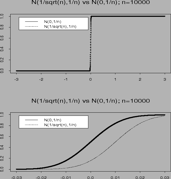
Q4) If
![]() is the distribution
of
is the distribution
of ![]() close to that of
close to that of ![]() ?
?
Answers depend on how close close needs to be so it's a matter of definition.
In practice the usual sort of approximation we want
to make is to say that some random variable ![]() , say,
has nearly some continuous distribution, like
, say,
has nearly some continuous distribution, like ![]() .
.
So: want to know probabilities like ![]() are nearly
are nearly
![]() .
.
Real difficulty: case of discrete random variables or infinite dimensions: not done in this course.
Mathematicians' meaning of close:
Either they can provide an upper bound on the distance between the two things or they are talking about taking a limit.
In this course we take limits.
Definition: A sequence of random variables ![]() converges in
distribution to a random variable
converges in
distribution to a random variable ![]() if
if
Now let's go back to the questions I asked:


Summary: to derive approximate distributions:
Show sequence of rvs ![]() converges to some
converges to some ![]() .
.
The limit distribution (i.e. dstbon of ![]() ) should
be non-trivial, like say
) should
be non-trivial, like say ![]() .
.
Don't say: ![]() is approximately
is approximately
![]() .
.
Do say:
![]() converges to
converges to ![]() in distribution.
in distribution.
The Central Limit Theorem
If
![]() are iid with mean 0 and variance 1 then
are iid with mean 0 and variance 1 then
![]() converges in distribution to
converges in distribution to ![]() . That is,
. That is,

Proof: As before
Multivariate convergence in distribution
Definition:
![]() converges in distribution to
converges in distribution to ![]() if
if
This is equivalent to either of
Cramér Wold Device:
![]() converges in distribution to
converges in distribution to ![]() for each
for each ![]()
or
Convergence of characteristic functions:
Extensions of the CLT
Slutsky's Theorem: If ![]() converges in distribution to
converges in distribution to ![]() and
and ![]() converges in distribution (or in probability) to
converges in distribution (or in probability) to ![]() , a
constant, then
, a
constant, then ![]() converges in distribution to
converges in distribution to ![]() . More
generally, if
. More
generally, if ![]() is continuous then
is continuous then
![]() .
.
Warning: the hypothesis that the limit of ![]() be constant is essential.
be constant is essential.
Definition: We say ![]() converges to
converges to ![]() in probability if
in probability if
The fact is that for ![]() constant convergence in distribution and in
probability are the same. In general convergence in probability implies
convergence in distribution. Both of these are weaker than almost sure
convergence:
constant convergence in distribution and in
probability are the same. In general convergence in probability implies
convergence in distribution. Both of these are weaker than almost sure
convergence:
Definition: We say ![]() converges to
converges to ![]() almost surely if
almost surely if
The delta method: Suppose:
If
![]() and
and
![]() then
then ![]() is
is
![]() matrix of first derivatives of components of
matrix of first derivatives of components of ![]() .
.
Example: Suppose
![]() are a sample from a population with
mean
are a sample from a population with
mean ![]() , variance
, variance ![]() , and third and fourth central moments
, and third and fourth central moments
![]() and
and ![]() . Then
. Then
Take
![]() .
Then
.
Then ![]() converges to
converges to
![]() .
Take
.
Take
![]() . Then
. Then
![$\displaystyle \Sigma = \left[\begin{array}{cc} \mu_4-\sigma^4 & \mu_3 -\mu(\mu^2+\sigma^2)\\
\mu_3-\mu(\mu^2+\sigma^2) & \sigma^2 \end{array} \right]
$](img103.gif)
Define
![]() .
Then
.
Then
![]() . The gradient of
. The gradient of ![]() has components
has components
![]() . This leads to
. This leads to
![\begin{multline*}
n^{1/2}(s^2-\sigma^2) \approx
\\
n^{1/2}[1, -2\mu]
\left[\b...
...ne{X^2} -
(\mu^2 + \sigma^2)
\\
\bar{X} -\mu
\end{array}\right]
\end{multline*}](img107.gif)
Remark: In this sort of problem it is best to learn to recognize that the
sample variance is unaffected by subtracting ![]() from each
from each ![]() . Thus
there is no loss in assuming
. Thus
there is no loss in assuming ![]() which simplifies
which simplifies ![]() and
and ![]() .
.
Special case: if the observations are
![]() then
then ![]() and
and
![]() . Our calculation has
. Our calculation has
