Postscript version of this page

STAT 801: Mathematical Statistics

Likelihood Methods of Inference

Toss coin 6 times and get Heads twice.

$p$ is probability of getting H.

Probability of getting exactly 2 heads is

$$15p^2(1-p)^4$$

This function of $p$, is likelihood function.

Definition: The likelihood function is map $L$: domain $\Theta$, values given by

$$L(\theta) = f_\theta(X)$$

Key Point: think about how the density depends on $\theta$ not about how it depends on $X$.

Notice: $X$, observed value of the data, has been plugged into the formula for density.

Notice: coin tossing example uses the discrete density for $f$.

We use likelihood for most inference problems:

1. Point estimation: we must compute an estimate $\hat\theta = \hat\theta(X)$ which lies in $\Theta$. The maximum likelihood estimate (MLE) of $\theta$ is the value $\hat\theta$ which maximizes $L(\theta)$ over $\theta\in \Theta$ if such a $\hat\theta$ exists.

2. Point estimation of a function of $\theta$: we must compute an estimate $\hat\phi = \hat\phi(X)$ of $\phi=g(\theta)$. We use $\hat\phi=g(\hat\theta)$ where $\hat\theta$ is the MLE of $\theta$.

3. Interval (or set) estimation. We must compute a set $C=C(X)$ in $\Theta$ which we think will contain $\theta_0$. We will use
   $$\{\theta\in\Theta: L(\theta) > c\}$$
   for a suitable $c$.

4. Hypothesis testing: decide whether or not $\theta_0\in\Theta_0$ where $\Theta_0 \subset \Theta$. We base our decision on the likelihood ratio
   $$\frac{\sup\{L(\theta); \theta \in \Theta_0\}}{ \sup\{L(\theta); \theta \in \Theta\setminus\Theta_0\}}$$

Maximum Likelihood Estimation

To find MLE maximize $L$.

Typical function maximization problem:

Set gradient of $L$ equal to 0

Check root is maximum, not minimum or saddle point.

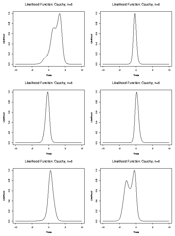
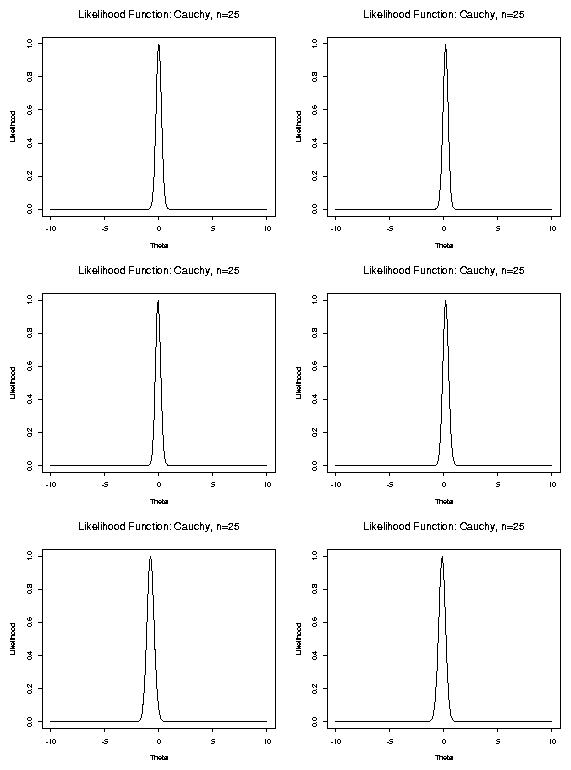
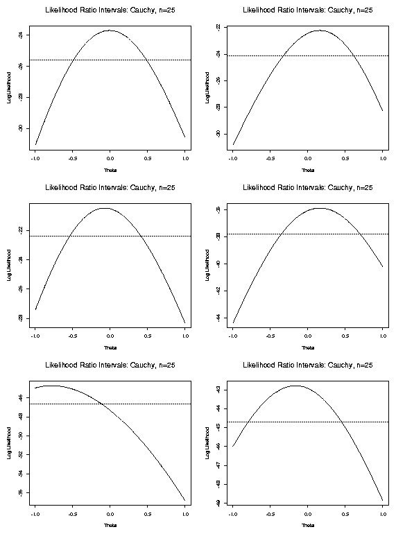
Examine some likelihood plots in examples:

Cauchy Data

Iid sample $X_1,\ldots,X_n$ from Cauchy$(\theta)$ density

$$f(x;\theta) = \frac{1}{\pi(1+(x-\theta)^2)}$$

The likelihood function is

$$L(\theta) = \prod_{i=1}^n\frac{1}{\pi(1+(X_i-\theta)^2)}$$

[Examine likelihood plots.]

<\CENTER> <\CENTER> <\CENTER> <\CENTER> I want you to notice the following points:

• The likelihood functions have peaks near the true value of $\theta$ (which is 0 for the data sets I generated).

• The peaks are narrower for the larger sample size.

• The peaks have a more regular shape for the larger value of $n$.

• I actually plotted $L(\theta)/L(\hat\theta)$ which has exactly the same shape as $L$ but runs from 0 to 1 on the vertical scale.

To maximize this likelihood: differentiate $L$, set result equal to 0.

Notice $L$ is product of $n$ terms; derivative is

$$\sum_{i=1}^n \prod_{j\neq i} \frac{1}{\pi(1+(X_j-\theta)^2)} \frac{2(X_i-\theta)}{\pi(1+(X_i-\theta)^2)^2}$$

which is quite unpleasant.

Much easier to work with logarithm of $L$: log of product is sum and logarithm is monotone increasing.

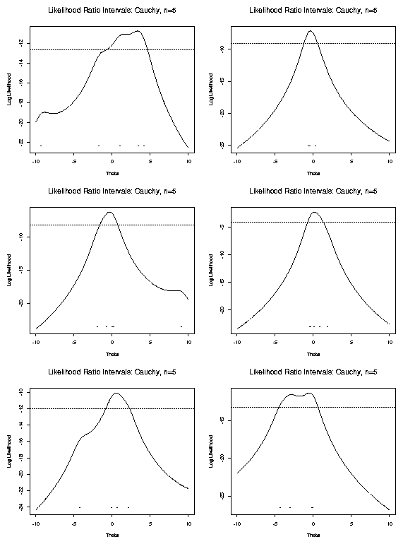
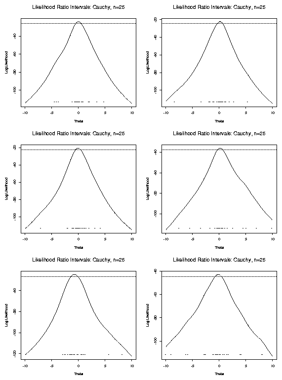
Definition: The Log Likelihood function is

$$\ell(\theta) = \log\{L(\theta)\} \, .$$

For the Cauchy problem we have

$$\ell(\theta)= -\sum \log(1+(X_i-\theta)^2) -n\log(\pi)$$

[Examine log likelihood plots.]

<\CENTER> <\CENTER> <\CENTER> <\CENTER> Notice the following points:

• Plots of $\ell$ for $n=25$ quite smooth, rather parabolic.

  
  

• For $n=5$ many local maxima and minima of $\ell$.

Likelihood tends to 0 as $\vert\theta\vert\to \infty$ so max of $\ell$ occurs at a root of $\ell^\prime$, derivative of $\ell$ wrt $\theta$.

Def'n: Score Function is gradient of $\ell$

$$U(\theta) = \frac{\partial\ell}{\partial\theta}$$

MLE $\hat\theta$ usually root of Likelihood Equations

$$U(\theta)=0$$

In our Cauchy example we find

$$U(\theta) = \sum \frac{2(X_i-\theta)}{1+(X_i-\theta)^2}$$

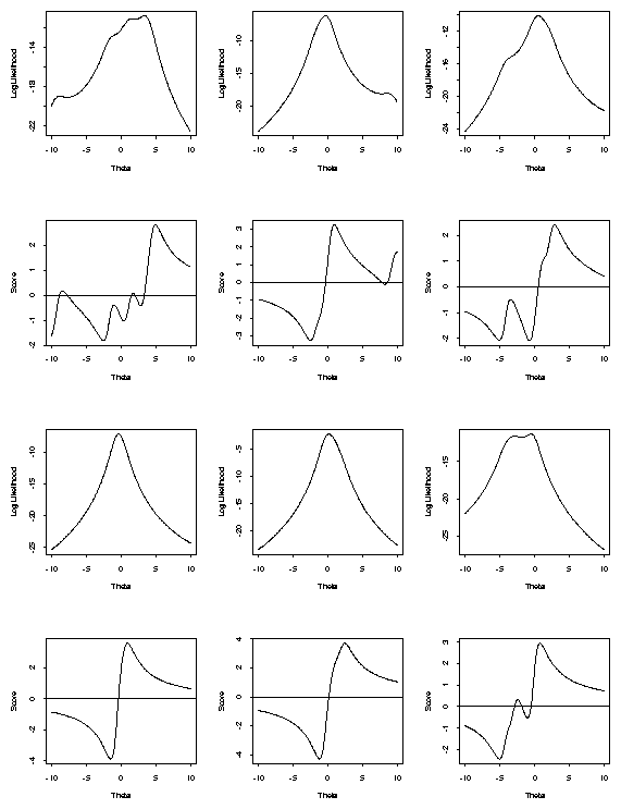
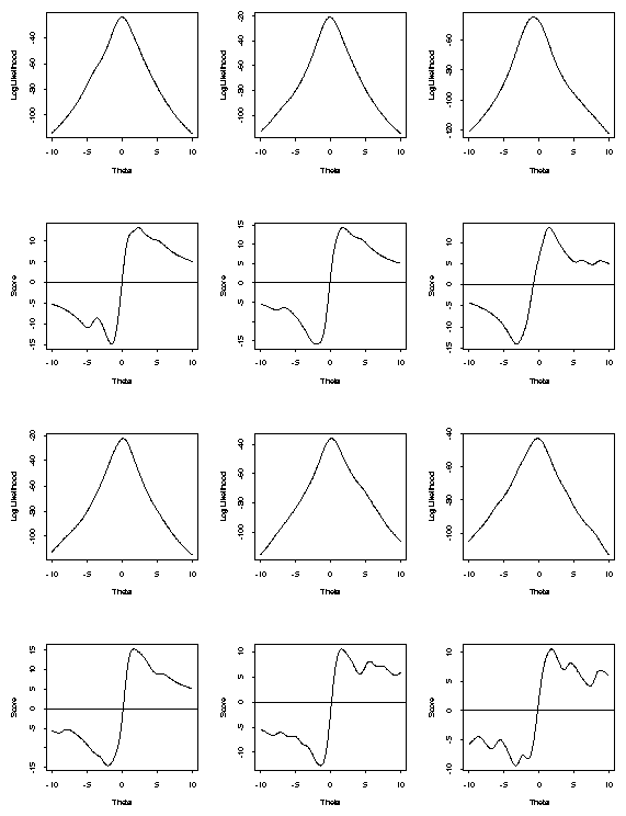
[Examine plots of score functions.]

Notice: often multiple roots of likelihood equations.

<\CENTER> <\CENTER> Example : $X\sim$ Binomial $(n,\theta)$

$$L(\theta) = \left( \! \! \! \begin{array}{c} n \\ X \end{array} \! \! \! \right) \theta^X (1-\theta)^{n-X}$$

$$\ell(\theta) = \log \!\!\left( \! \! \! \begin{array}{c} n \\ X \end{array} \! \! \! \right) +X \log(\theta) + (n-X) \log(1-\theta)$$

$$U(\theta) = \frac{X}{\theta} - \frac{n-X}{1-\theta}$$

The function $L$ is 0 at $\theta=0$ and at $\theta=1$ unless $X=0$ or $X=n$ so for $1 \le X \le n$ the MLE must be found by setting $U=0$ and getting

$$\hat\theta = \frac{X}{n}$$

For $X=n$ the log-likelihood has derivative

$$U(\theta) = \frac{n}{\theta} > 0$$

for all $\theta$ so that the likelihood is an increasing function of $\theta$ which is maximized at $\hat\theta=1=X/n$. Similarly when $X=0$ the maximum is at $\hat\theta=0=X/n$.

The Normal Distribution

Now we have $X_1,\ldots,X_n$ iid $N(\mu,\sigma^2)$. There are two parameters $\theta=(\mu,\sigma)$. We find

$$L(\mu,\sigma) = \frac{e^{-\sum(X_i-\mu)^2/(2\sigma^2)}}{ (2\pi)^{-n/2} \sigma^{-n}}$$

$$\ell(\mu,\sigma) = -\frac{n}{2}\log(2\pi) -\frac{\sum(X_i-\mu)^2}{2\sigma^2} -n\log(\sigma)$$

and that $U$ is

$$\left[ \begin{array}{c} \frac{\sum(X_i-\mu)}{\sigma^2} \\ \frac{\sum(X_i-\mu)^2}{\sigma^3} -\frac{n}{\sigma} \end{array}\right]$$

Notice that $U$ is a function with two components because $\theta$ has two components.

Setting the likelihood equal to 0 and solving gives

$$\hat\mu=\bar{X}$$

and

$$\hat\sigma = \sqrt{\frac{\sum(X_i-\bar{X})^2}{n}}$$

Check this is maximum by computing one more derivative. Matrix $H$ of second derivatives of $\ell$ is

$$\left[\begin{array}{cc} \frac{-n}{\sigma^2} & \frac{-2\sum(X_i-\m... ...3} & \frac{-3\sum(X_i-\mu)^2}{\sigma^4} +\frac{n}{\sigma^2} \end{array}\right]$$

Plugging in the mle gives

$$H(\hat\theta) = \left[\begin{array}{cc} \frac{-n}{\hat\sigma^2} & 0 \\ 0 & \frac{-2n}{\hat\sigma^2} \end{array}\right]$$

which is negative definite. Both its eigenvalues are negative. So $\hat\theta$ must be a local maximum.

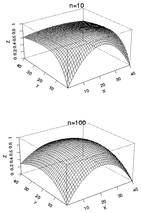
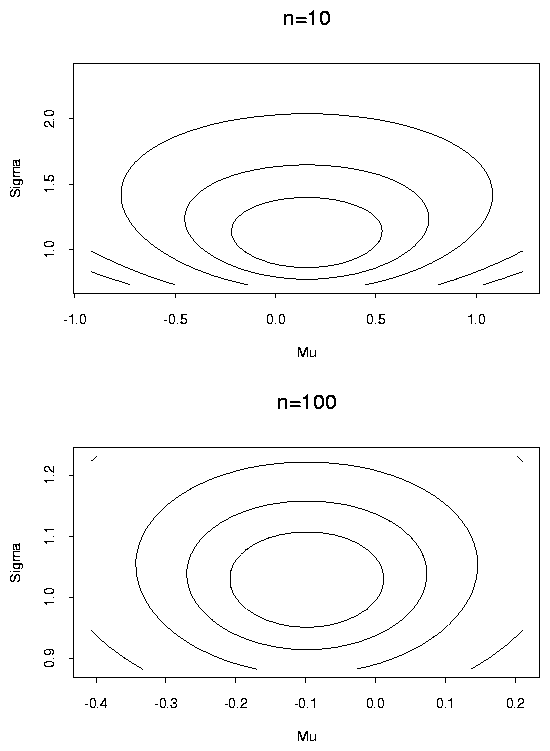
[Examine contour and perspective plots of $\ell$.]

<\CENTER> <\CENTER> Notice that the contours are quite ellipsoidal for the larger sample size.

For $X_1,\ldots,X_n$ iid log likelihood is

$$\ell(\theta )= \sum \log(f(X_i,\theta)) \, .$$

The score function is

$$U(\theta) = \sum \frac{\partial \log f}{\partial\theta}(X_i,\theta) \, .$$

MLE $\hat\theta$ maximizes $\ell$. If maximum occurs in interior of parameter space and the log likelihood continuously differentiable then $\hat\theta$ solves the likelihood equations

$$U(\theta) = 0 \, .$$

Some examples concerning existence of roots:

Solving $U(\theta)=0$: Examples

N $(\mu,\sigma^2$)

Unique root of likelihood equations is a global maximum.

[Remark: Suppose we called $\tau=\sigma^2$ the parameter. Score function still has two components: first component same as before but second component is

$$\frac{\partial}{\partial\tau} \ell = \frac{\sum(X_i-\mu)^2}{2\tau^2} -\frac{n}{2\tau}$$

Setting the new likelihood equations equal to 0 still gives

$$\hat\tau = \hat\sigma^2$$

General invariance (or equivariance) principal: If $\phi=g(\theta)$ is some reparametrization of a model (a one to one relabelling of the parameter values) then $\hat\phi=g(\hat\theta)$. Does not apply to other estimators.]

Cauchy: location $\theta$

At least 1 root of likelihood equations but often several more. One root is a global maximum; others, if they exist may be local minima or maxima.

Binomial($n,\theta$)

If $X=0$ or $X=n$: no root of likelihood equations; likelihood is monotone. Other values of $X$: unique root, a global maximum. Global maximum at $\hat\theta = X/n$ even if $X=0$ or $n$.

The 2 parameter exponential

The density is

$$f(x;\alpha,\beta) = \frac{1}{\beta} e^{-(x-\alpha)/\beta} 1(x>\alpha)$$

Log-likelihood is $-\infty$ for $\alpha > \min\{X_1,\ldots,X_n\}$ and otherwise is

$$\ell(\alpha,\beta) = -n\log(\beta) -\sum(X_i-\alpha)/\beta$$

Increasing function of $\alpha$ till $\alpha$ reaches

$$\hat\alpha = X_{(1)} = \min\{X_1,\ldots,X_n\}$$

which gives mle of $\alpha$. Now plug in $\hat\alpha$ for $\alpha$; get so-called profile likelihood for $\beta$:

$$\ell_{\mbox{profile}}(\beta) = -n\log(\beta) -\sum(X_i-X_{(1)})/\beta$$

Set $\beta$ derivative equal to 0 to get

$$\hat\beta =\sum(X_i-X_{(1)})/n$$

Notice mle $\hat\theta=(\hat\alpha,\hat\beta)$ does not solve likelihood equations; we had to look at the edge of the possible parameter space. $\alpha$ is called a support or truncation parameter. ML methods behave oddly in problems with such parameters.

Three parameter Weibull

The density in question is

$$f(x;\alpha,\beta,\gamma) = \frac{1}{\beta} \left(\frac{x-\alpha}{\beta}\right)^{\gamma-1} \exp[-\{(x-\alpha)/\beta\}^\gamma]1(x>\alpha)$$

Three likelihood equations:

Set $\beta$ derivative equal to 0; get

$$\hat\beta(\alpha,\gamma) = \left[\sum (X_i-\alpha)^\gamma/n\right]^{1/\gamma}$$

where $\hat\beta(\alpha,\gamma)$ indicates mle of $\beta$ could be found by finding the mles of the other two parameters and then plugging in to the formula above. It is not possible to find explicitly the remaining two parameters; numerical methods are needed.

However putting $\gamma < 1$ and letting $\alpha \to X_{(1)}$ will make the log likelihood go to $\infty$.

MLE is not uniquely defined: any $\gamma < 1$ and any $\beta$ will do.

If the true value of $\gamma$ is more than 1 then the probability that there is a root of the likelihood equations is high; in this case there must be two more roots: a local maximum and a saddle point! For a true value of $\gamma>1$ the theory we detail below applies to the local maximum and not to the global maximum of the likelihood equations.