STAT 802: Multivariate Analysis

Course outline:

Basic structure of typical multivariate data set:

Case by variables: data in matrix. Each row is a case, each column is a variable.

Example: Fisher's iris data: 5 rows of 150 by 5 matrix:

Case Sepal Sepal Petal Petal
# Variety Length Width Length Width
1 Setosa 5.1 3.5 1.4 0.2
2 Setosa 4.9 3.0 1.4 0.2
&vellip#vdots; &vellip#vdots; &vellip#vdots; &vellip#vdots; &vellip#vdots; &vellip#vdots;
51 Versicolor 7.0 3.2 4.7 1.4
&vellip#vdots; &vellip#vdots; &vellip#vdots; &vellip#vdots; &vellip#vdots; &vellip#vdots;
Usual model: rows of data matrix are independent random variables.

Vector valued random variable: function $ {\bf X}:\Omega\mapsto \mathbb {R}^p$ such that, writing $ {\bf X}=(X_1,\ldots,X_p)^T$,

$\displaystyle P(X_1 \le x_1, \ldots , X_p \le x_p)
$

defined for any const's $ (x_1,\ldots,x_p)$.

Cumulative Distribution Function (CDF) of $ {\bf X}$: function $ F_{\bf X}$ on $ \mathbb {R}^p$ defined by

$\displaystyle F_{\bf X}(x_1,\ldots, x_p) =
P(X_1 \le x_1, \ldots , X_p \le x_p) \,.
$

Defn: Distribution of rv $ {\bf X}$ is absolutely continuous if there is a function $ f$ such that

$\displaystyle P({\bf X}\in A) = \int_A f(x) dx$ (1)

for any (Borel) set $ A$. This is a $ p$ dimensional integral in general. Equivalently

\begin{multline*}
F(x_1,\ldots,x_p) = \\
\int_{-\infty}^{x_1}\cdots
\int_{-\infty}^{x_p} f(y_1,\ldots,y_p) \, dy_p,\ldots,dy_1 \,.
\end{multline*}

Defn: Any $ f$ satisfying ([*]) is a density of $ {\bf X}$.

For most $ x$ $ F$ is differentiable at $ x$ and

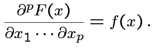
$\displaystyle \frac{\partial^pF(x) }{\partial x_1\cdots \partial x_p} =f(x) \,.
$

Building Multivariate Models

Basic tactic: specify density of

$\displaystyle {\bf X}=(X_1,\ldots, X_p)^T.$

Tools: marginal densities, conditional densities, independence, transformation.

Marginalization: Simplest multivariate problem

$\displaystyle {\bf X}=(X_1,\ldots,X_p), \qquad Y=X_1$

(or in general $ Y$ is any $ X_j$).

Theorem 1   If $ {\bf X}$ has density $ f(x_1,\ldots,x_p)$ and $ q<p$ then $ {\bf Y}=(X_1,\ldots,X_q)$ has density

\begin{multline*}
f_{\bf Y}(x_1,\ldots,x_q)
=
\\
\int_{-\infty}^\infty \cdots \int_{-\infty}^\infty
f(x_1,\ldots,x_p) \, dx_{q+1} \ldots dx_p
\end{multline*}

$ f_{X_1,\ldots,X_q}$ is the marginal density of $ X_1,\ldots,X_q$ and $ f_{\bf X}$ the joint density of $ {\bf X}$ but they are both just densities. ``Marginal'' just to distinguish from the joint density of $ {\bf X}$.

Independence, conditional distributions

Def'n: Events $ A$ and $ B$ are independent if

$\displaystyle P(AB) = P(A)P(B) \,.
$

(Notation: $ AB$ is the event that both $ A$ and $ B$ happen, also written $ A\cap B$.)


Def'n: $ A_i$, $ i=1,\ldots,p$ are independent if

$\displaystyle P(A_{i_1} \cdots A_{i_r}) = \prod_{j=1}^r P(A_{i_j})
$

for any $ 1 \le i_1 < \cdots < i_r \le p$.

Def'n: $ {\bf X}$ and $ {\bf Y}$ are independent if

$\displaystyle P({\bf X}\in A; {\bf Y}\in B) = P({\bf X}\in A)P({\bf Y}\in B)
$

for all $ A$ and $ B$.

Def'n: Rvs $ {\bf X}_1,\ldots,{\bf X}_p$ independent:

$\displaystyle P({\bf X}_1 \in A_1, \cdots , {\bf X}_p \in A_p ) = \prod P({\bf X}_i \in A_i)
$

for any $ A_1,\ldots,A_p$.

Theorem:

  1. If $ {\bf X}$ and $ {\bf Y}$ are independent with joint density $ f_{{\bf X},{\bf Y}}(x,y)$ then $ {\bf X}$ and $ {\bf Y}$ have densities $ f_{\bf X}$ and $ f_{\bf Y}$, and

    $\displaystyle f_{{\bf X},{\bf Y}}(x,y) = f_{\bf X}(x) f_{\bf Y}(y) \,.
$


  2. If $ {\bf X}$ and $ {\bf Y}$ independent with marginal densities $ f_{\bf X}$ and $ f_{\bf Y}$ then $ ({\bf X},{\bf Y})$ has joint density

    $\displaystyle f_{{\bf X},{\bf Y}}(x,y) = f_{\bf X}(x) f_{\bf Y}(y) \,.
$


  3. If $ ({\bf X},{\bf Y})$ has density $ f(x,y)$ and there exist $ g(x)$ and $ h(y)$ st $ f(x,y) = g(x) h(y)
$ for (almost) all $ (x,y)$ then $ {\bf X}$ and $ {\bf Y}$ are independent with densities given by

    $\displaystyle f_{\bf X}(x) = g(x)/\int_{-\infty}^\infty g(u) du
$

    $\displaystyle f_{\bf Y}(y) = h(y)/\int_{-\infty}^\infty h(u) du \,.
$

Theorem: If $ {\bf X}_1,\ldots,{\bf X}_p$ are independent and $ {\bf Y}_i =g_i({\bf X}_i)$ then $ {\bf Y}_1,\ldots,{\bf Y}_p$ are independent. Moreover, $ ({\bf X}_1,\ldots,{\bf X}_q)$ and $ ({\bf X}_{q+1},\ldots,{\bf X}_{p})$ are independent.

Conditional densities

Conditional density of $ {\bf Y}$ given $ {\bf X}=x$:

$\displaystyle f_{{\bf Y}\vert{\bf X}}(y\vert x) = f_{{\bf X},{\bf Y}}(x,y)/f_{\bf X}(x) \, ;
$

in words ``conditional = joint/marginal''.

Change of Variables

Suppose $ {\bf Y}=g({\bf X}) \in \mathbb {R}^p$ with $ {\bf X}\in \mathbb {R}^p$ having density $ f_{\bf X}$. Assume $ g$ is a one to one (``injective") map, i.e., $ g(x_1) = g(x_2)$ if and only if $ x_1 = x_2$. Find $ f_{\bf Y}$:

Step 1: Solve for $ x$ in terms of $ y$: $ x=g^{-1}(y)$.

Step 2: Use basic equation:

$\displaystyle f_{\bf Y}(y) dy =f_{\bf X}(x) dx
$

and rewrite it in the form

$\displaystyle f_{\bf Y}(y) = f_{\bf X}(g^{-1}(y)) \frac{dx}{dy}
$

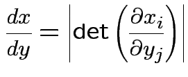
Interpretation of derivative $ \frac{dx}{dy}$ when $ p>1$:

$\displaystyle \frac{dx}{dy} = \left\vert \mbox{det}\left(\frac{\partial x_i}{\partial y_j}\right)\right\vert
$

which is the so called Jacobian.

Equivalent formula inverts the matrix:

$\displaystyle f_{\bf Y}(y) = \frac{f_{\bf X}(g^{-1}(y))}{ \left\vert\frac{dy}{dx}\right\vert} \,.
$

This notation means

$\displaystyle \left\vert\frac{dy}{dx}\right\vert =
\left\vert \mbox{det} \left...
...} & \cdots &
\frac{\partial y_p}{\partial x_p}
\end{array} \right]\right\vert
$

but with $ x$ replaced by the corresponding value of $ y$, that is, replace $ x$ by $ g^{-1}(y)$.

Example: The density

$\displaystyle f_{\bf X}(x_1,x_2) = \frac{1}{2\pi} \exp\left\{ -\frac{x_1^2+x_2^2}{2}\right\}
$

is the standard bivariate normal density. Let $ {\bf Y}=(Y_1,Y_2)$ where $ Y_1=\sqrt{X_1^2+X_2^2}$ and $ 0 \le Y_2< 2\pi$ is angle from the positive $ x$ axis to the ray from the origin to the point $ (X_1,X_2)$. I.e., $ {\bf Y}$ is $ {\bf X}$ in polar co-ordinates.

Solve for $ x$ in terms of $ y$:

$\displaystyle X_1$ $\displaystyle =$ $\displaystyle Y_1 \cos(Y_2)$  
$\displaystyle X_2$ $\displaystyle =$ $\displaystyle Y_1 \sin(Y_2)$  

so that
$\displaystyle g(x_1,x_2)$ $\displaystyle =$ $\displaystyle (g_1(x_1,x_2),g_2(x_1,x_2))$  
       
  $\displaystyle =$ $\displaystyle (\sqrt{x_1^2 + x_2^2},$argument$\displaystyle (x_1,x_2))$  
       
$\displaystyle g^{-1}(y_1,y_2)$ $\displaystyle =$ $\displaystyle (g^{-1}_1(y_1,y_2),g^{-1}_2(y_1,y_2))$  
       
  $\displaystyle =$ $\displaystyle (y_1\cos(y_2), y_1\sin(y_2))$  
       
$\displaystyle \left\vert\frac{dx}{dy}\right\vert$ $\displaystyle =$ $\displaystyle \left\vert \mbox{det}\left( \begin{array}{cc}
\cos(y_2) & -y_1\sin(y_2)
\\
\\
\sin(y_2) & y_1 \cos(y_2)
\end{array}\right) \right\vert$  
       
  $\displaystyle =$ $\displaystyle y_1 \,.$  

It follows that
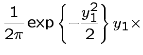
$\displaystyle f_{\bf Y}(y_1,y_2)$ $\displaystyle =$ $\displaystyle \frac{1}{2\pi}\exp\left\{-\frac{y_1^2}{2}\right\}y_1 \times$  
       
    $\displaystyle 1(0 \le y_1 < \infty)
1(0 \le y_2 < 2\pi ) \,.$  

Next: marginal densities of $ Y_1$, $ Y_2$?

Factor $ f_{\bf Y}$ as $ f_{\bf Y}(y_1,y_2) = h_1(y_1)h_2(y_2)$ where

$\displaystyle h_1(y_1) = y_1e^{-y_1^2/2} 1(0 \le y_1 < \infty)
$

and

$\displaystyle h_2(y_2) = 1(0 \le y_2 < 2\pi )/ (2\pi) \,.
$

Then

$\displaystyle f_{Y_1}(y_1)$ $\displaystyle =$ $\displaystyle \int_{-\infty}^\infty h_1(y_1)h_2(y_2) \, dy_2$  
  $\displaystyle =$ $\displaystyle h_1(y_1) \int_{-\infty}^\infty h_2(y_2) \, dy_2$  

so marginal density of $ Y_1$ is a multiple of $ h_1$. Multiplier makes $ \int f_{Y_1} =1$ but in this case

$\displaystyle \int_{-\infty}^\infty h_2(y_2) \, dy_2 = \int_0^{2\pi} (2\pi)^{-1} dy_2 = 1
$

so that

$\displaystyle f_{Y_1}(y_1) = y_1e^{-y_1^2/2} 1(0 \le y_1 < \infty) \,.
$

(Special Weibull or Rayleigh distribution.) Similarly

$\displaystyle f_{Y_2}(y_2) = 1(0 \le y_2 < 2\pi )/ (2\pi)
$

which is the Uniform$ (0,2\pi)$ density. Exercise: $ W=Y_1^2/2$ has standard exponential distribution. Recall: by definition $ U=Y_1^2$ has a $ \chi^2$ distribution on 2 degrees of freedom. Exercise: find $ \chi^2_2$ density.

Remark: easy to check $ \int_0^\infty ye^{-y^2/2} dy = 1$.

Thus: have proved original bivariate normal density integrates to 1.

Put $ I=\int_{-\infty}^\infty e^{-x^2/2} dx$. Get

$\displaystyle I^2$ $\displaystyle = \int_{-\infty}^\infty e^{-x^2/2} dx \int_{-\infty}^\infty e^{-y^2/2} dy$    
  $\displaystyle = \int_{-\infty}^\infty \int_{-\infty}^\infty e^{-(x^2+y^2)/2} dydx$    
  $\displaystyle = 2\pi.$    

So $ I=\sqrt{2\pi}$.


Richard Lockhart
2002-09-25