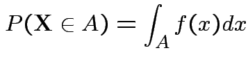
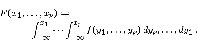
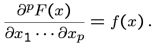
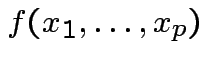
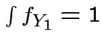
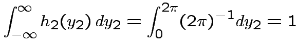
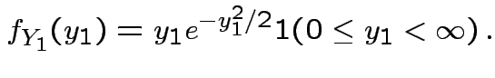
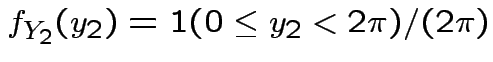
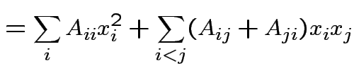
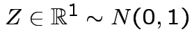
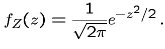
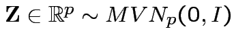
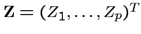
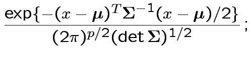
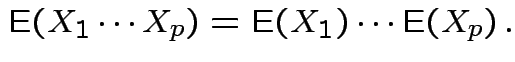
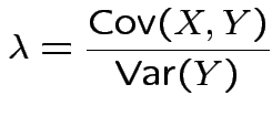
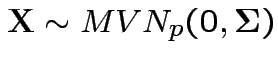
 ,
,
Course outline:
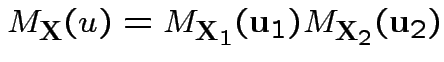
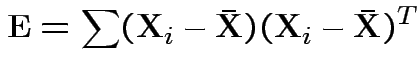
Basic structure of typical multivariate data set:
Case by variables: data in matrix. Each row is a case, each column is a variable.
Example: Fisher's iris data: 5 rows of 150 by 5 matrix:
| Case | Sepal | Sepal | Petal | Petal | |
| # | Variety | Length | Width | Length | Width |
| 1 | Setosa | 5.1 | 3.5 | 1.4 | 0.2 |
| 2 | Setosa | 4.9 | 3.0 | 1.4 | 0.2 |
| &vellip#vdots; | &vellip#vdots; | &vellip#vdots; | &vellip#vdots; | &vellip#vdots; | &vellip#vdots; |
| 51 | Versicolor | 7.0 | 3.2 | 4.7 | 1.4 |
| &vellip#vdots; | &vellip#vdots; | &vellip#vdots; | &vellip#vdots; | &vellip#vdots; | &vellip#vdots; |
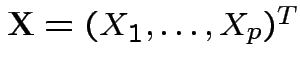
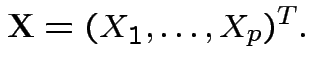
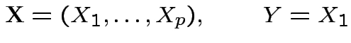
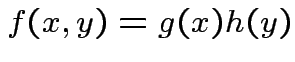
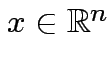
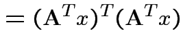
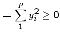
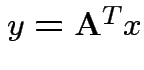
Vector valued random variable: function
![]() such that,
writing
,
such that,
writing
,
 .
.
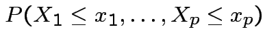
Cumulative Distribution Function (CDF) of ![]() : function
: function  on
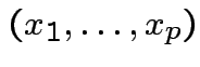
on
![]() defined by
defined by

Defn: Distribution of rv ![]() is absolutely continuous
if there is a function
is absolutely continuous
if there is a function ![]() such that
such that
Defn: Any ![]() satisfying (1) is a density of
satisfying (1) is a density of ![]() .
.
For most ![]()
![]() is differentiable at
is differentiable at ![]() and
and
Basic tactic: specify density of
Tools: marginal densities, conditional densities, independence, transformation.
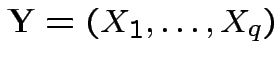
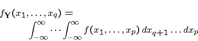
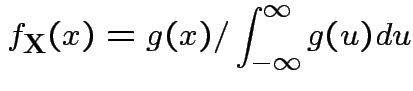
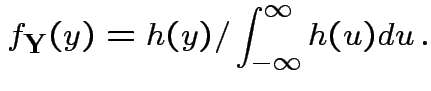
Marginalization: Simplest multivariate problem
 ).
).
 and
and  then
then
 has density
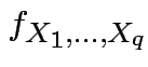 is the marginal density of
 and
and ![]() the joint density of
the joint density of ![]() but
they are both just densities.
``Marginal'' just to
distinguish from the joint density of
but
they are both just densities.
``Marginal'' just to
distinguish from the joint density of ![]() .
.
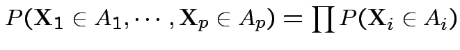
Def'n: Events ![]() and
and ![]() are independent if
are independent if
Def'n: ![]() ,
,
 are
independent if
are
independent if
 .
.
Def'n: ![]() and
and ![]() are
independent if
are
independent if

Def'n: Rvs
 independent:
 .
.
Theorem:
 then
then 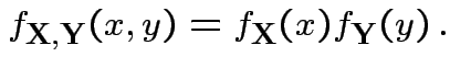
 has joint density
has density  and there exist
 and
and  st
st
 for (almost) all
  then
then
Theorem: If
are independent and
 then
then
 are independent.
Moreover,
are independent.
Moreover,
 and
and
 are
independent.
are
independent.
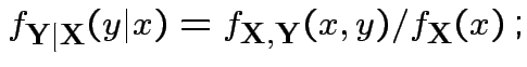
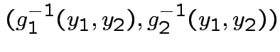
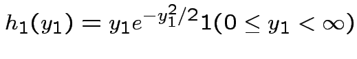
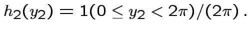
Conditional density of ![]() given
given ![]() :
:
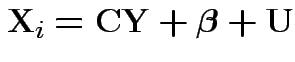
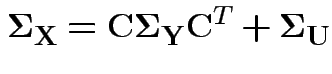
Suppose
 with
with
 having density
 ![]() .
Assume
.
Assume ![]() is a one to one (``injective") map, i.e.,
is a one to one (``injective") map, i.e.,
 if and only if
  .
Find
.
Find ![]() :
:
Step 1: Solve for ![]() in terms of
in terms of ![]() :
:
 .
.
Step 2: Use basic equation:
 :
:
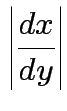
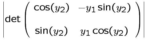
Equivalent formula inverts the matrix:
![$\displaystyle \left\vert\frac{dy}{dx}\right\vert =
\left\vert \mbox{det} \left...
...} & \cdots &
\frac{\partial y_p}{\partial x_p}
\end{array} \right]\right\vert
$](img71.gif)
 .
.
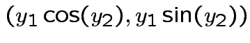
Example: The density
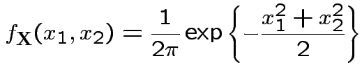
 where
where
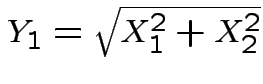 and
and
 is angle
from the positive
is angle
from the positive  .
I.e.,
.
I.e.,
Solve for ![]() in terms of
in terms of ![]() :
:
 |
 |
||
 |
 |
 |
 |
||
 argument argument |
|||
 |
 |
||
 |
|||
 |
 |
||
 |
 |
 |
||
 |
Next: marginal densities of ![]() ,
, ![]() ?
?
Factor ![]() as
as
 where
where
Then
 |
 |
||
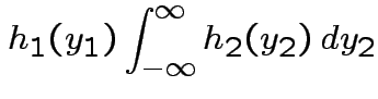 |
 but in this case
 density.
Exercise:
density.
Exercise:  has standard exponential
distribution. Recall: by definition
has standard exponential
distribution. Recall: by definition  has a
has a
Remark: easy to check
 .
.
Thus: have proved original bivariate normal density integrates to 1.
Put
 .
Get
.
Get
 |
||
 |
||
 |
 .
.
Notation:
 are column vectors
![$\displaystyle x=\left[\begin{array}{c} x_1 \\ \vdots \\ x_n \end{array}\right]
$](img122.gif)
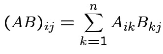
 matrix
  .
.

and  then
then  matrix
 which is an
 matrix with
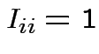 for all
  for any pair
 is called the identity matrix.
 is the
set of all vectors
is the
set of all vectors  . It is a vector space.
The column space of a matrix,
. It is a vector space.
The column space of a matrix,
is linearly independent
if
 implies
  for all
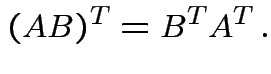
Defn: The transpose, ![]() , of an matrix
, of an matrix ![]() is
the
is
the
 matrix whose entries are given by
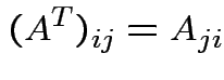 . We have
Defn: rank of matrix ![]() ,
rank
,
rank :
# of linearly independent
columns of
:
# of linearly independent
columns of ![]() .
We have
.
We have
rank |
||
 |
If ![]() is
then
rank
is
then
rank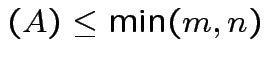 .
.
For now: all matrices square
.
If there is a matrix ![]() such that
such that
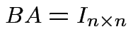 then
we call
then
we call ![]() the inverse of
the inverse of ![]() . If
. If ![]() exists it is unique and
exists it is unique and
![]() and we write
and we write ![]() . The matrix
. The matrix ![]() has an inverse if and only
if
rank
has an inverse if and only
if
rank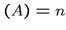 .
.
Inverses have the following properties:
Again ![]() is . The determinant if a function on the set
of
matrices such that:
is . The determinant if a function on the set
of
matrices such that:
 .
.
 det
det
 .)
.)
is a linear function of each column of  with
with det |
 |
|
det |
||
 |
Here are some properties of the determinant:
 det.
det.
 detdet
 .
.
 det.
det.
 if and only if
rank.
if and only if
rank.
implies  .
.
Defn: Two vectors ![]() and
and ![]() are orthogonal if
are orthogonal if
 .
.
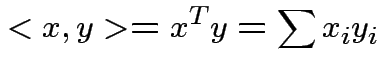
Defn: The inner product or dot product of ![]() and
and ![]() is
is
Defn: ![]() and
and ![]() are orthogonal if
are orthogonal if  .
.
Defn: The norm (or length) of ![]() is
is
![]() is orthogonal if each column of
is orthogonal if each column of ![]() has length 1 and
is orthogonal to each other column of
has length 1 and
is orthogonal to each other column of ![]() .
.
Suppose ![]() is an
matrix. The function
is an
matrix. The function
 |
 |
|
 |
depends only on the total
 . In
fact
. In
fact
If ![]() is
and
is
and
 and
and
 such that
 matrix
 is singular.
Therefore
det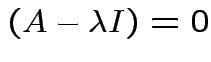 .
.
Conversely: if
singular
then there is  such that
 .
.
Fact:
det is polynomial in
 ![]() of degree
of degree
![]() .
.
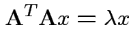
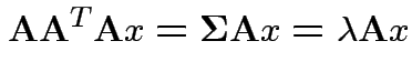
Each root is an eigenvalue.
General ![]() the roots could be
multiple roots or complex valued.
the roots could be
multiple roots or complex valued.
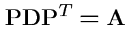
Matrix ![]() is diagonalized by a non-singular matrix
is diagonalized by a non-singular matrix
![]() if
if
![]() is diagonal.
is diagonal.
If so then ![]() so each column of
so each column of ![]() is eigenvector of
is eigenvector of ![]() with
the
with
the ![]() th column having eigenvalue
th column having eigenvalue  .
.
Thus to be diagonalizable
![]() must have
must have ![]() linearly independent eigenvectors.
linearly independent eigenvectors.
If ![]() is symmetric then
is symmetric then
 are two eigenvalues of
 |
 |
|
 |
 and
we see
and
we see
 . Eigenvectors corresponding
to distinct eigenvalues are orthogonal.
. Eigenvectors corresponding
to distinct eigenvalues are orthogonal.
Defn: A symmetric matrix ![]() is non-negative definite if
is non-negative definite if
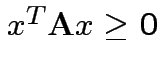 for all
 ![]() . It is positive definite if in addition
. It is positive definite if in addition
![]() implies
implies
![]() .
.
![]() is non-negative definite iff all its eigenvalues are
non-negative.
is non-negative definite iff all its eigenvalues are
non-negative.
![]() is positive definite iff all eigenvalues positive.
is positive definite iff all eigenvalues positive.
A non-negative definite matrix has a symmetric non-negative definite square root. If
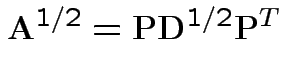
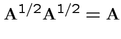
 .
.
Suppose ![]() vector subspace of
vector subspace of
![]() ,
,
 basis for
 ![]() . Given any
there
is a unique
. Given any
there
is a unique  which is closest to
 ![]() ;
; ![]() minimizes
minimizes
 . Any
. Any 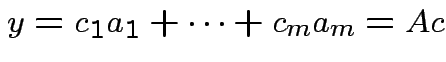 , columns
;
, columns
;
 |
||
 |
||
 |
||
 |
||
 |
Note that
 and that
 we see that
 |
 |
|
 |
||
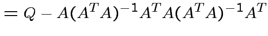 |
||
 |
 |
 |
|
 |
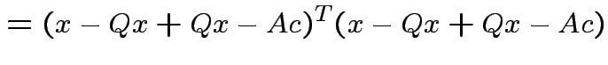
Choose ![]() to minimize:
minimize second term.
to minimize:
minimize second term.
Achieved by making
 .
.
Since
 can
take
can
take
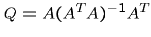
Summary:
closest point ![]() in
in ![]() is
is
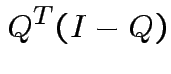
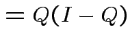
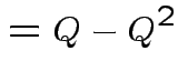
Notice that the matrix ![]() is idempotent:
is idempotent:
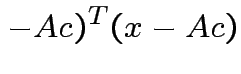
 the orthogonal projection of is perpendicular to the residual
.
the orthogonal projection of is perpendicular to the residual
.
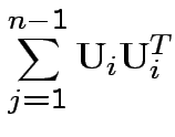
Suppose 
 matrix,
 ,
, 
 and
and 
 . Make
 matrix
by putting in 2 by 2 matrix:
matrix
by putting in 2 by 2 matrix:
![$\displaystyle A = \left[ \begin{array}{cc}
A_{11} & A_{12}
\\
A_{21} & A_{22}
\end{array}\right]
$](img279.gif)
![$\displaystyle A_{11} = \left[ \begin{array}{cc} 1 & 0 \\ 0 & 1 \end{array}\right]
$](img280.gif)
![$\displaystyle A_{12} = \left[ \begin{array}{c} 2 \\ 3 \end{array}\right]
$](img281.gif)
![$\displaystyle A_{21} = \left[ \begin{array}{cc} 4 & 5\end{array}\right]
$](img282.gif)
![$\displaystyle A_{22} = \left[ 6 \right]
$](img283.gif)
![$\displaystyle A = \left[ \begin{array}{cc\vert c}
1 & 0 & 2
\\
0 & 1 & 3
\\
\hline
4 & 5 & 6
\end{array}\right]
$](img284.gif)
We can work with partitioned matrices just like ordinary matrices always making sure that in products we never change the order of multiplication of things.
![$\displaystyle \left[ \begin{array}{cc} A_{11} & A_{12} \\ \\ A_{21} & A_{22} \end{array} \right]$](img285.gif) |
![$\displaystyle + \left[ \begin{array}{cc} B_{11} & B_{12} \\ \\ B_{21} & B_{22} \end{array} \right]$](img286.gif) |
|
![$\displaystyle \left[ \begin{array}{cc} A_{11}+B_{11} & A_{12}+B_{12} \\ \\ A_{21}+B_{21} & A_{22}+B_{22} \end{array} \right]$](img287.gif) |
![\begin{multline*}
\left[ \begin{array}{cc}
A_{11} & A_{12}
\\
\\
A_{21} & A_{2...
...{11}+A_{22}B_{21} &A_{21}B_{12}+ A_{22}B_{22}
\end{array}\right]
\end{multline*}](img288.gif)
Note partitioning of ![]() and
and ![]() must match.
must match.
Addition: dimensions of and  must be the same.
Multiplication formula  must
have as many columns as
must
have as many columns as  has rows, etc.
In general:
need
 to make sense for each
  .
.
Works with more than a 2 by 2 partitioning.
Defn: block diagonal matrix: partitioned matrix ![]() for which if . If
for which if . If
![$\displaystyle A = \left[ \begin{array}{cc}
A_{11} & 0
\\
0 & A_{22}
\end{array}\right]
$](img294.gif)
 is invertible and
then
is invertible and
then
![$\displaystyle A^{-1} = \left[ \begin{array}{cc}
A_{11}^{-1} & 0
\\
0 & A_{22}^{-1}
\end{array}\right]
$](img296.gif)
 det
det det
det .
Similar formulas work for larger matrices.
.
Similar formulas work for larger matrices.
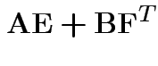
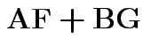
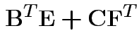
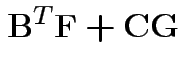
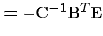
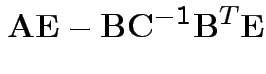
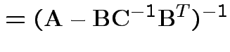
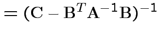
Partitioned inverses. Suppose ![]() ,
, ![]() are symmetric positive
definite. Look for inverse of
are symmetric positive
definite. Look for inverse of
![$\displaystyle \left[\begin{array}{cc} {\bf A}& {\bf B}\\ {\bf B}^T & {\bf C}\end{array}\right]
$](img301.gif)
![$\displaystyle \left[\begin{array}{cc} {\bf E}& {\bf F}\\ {\bf F}^T & {\bf G}\end{array}\right]
$](img302.gif)
 |
 |
|
 |
 |
|
 |
|
|
 |
|
Solve to get
 |
 |
|
 |
|
|
 |
||
 |
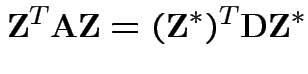
Defn:
 iff
iff
Defn:
 if and only if
 with the
![]() independent and each
independent and each
 .
.
In this case according to our theorem
 |
 |
|
 |
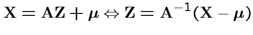
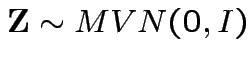
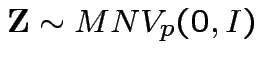
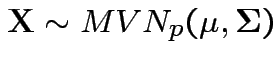
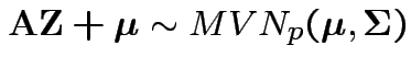
Defn:
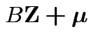
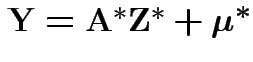
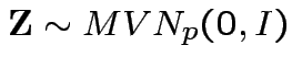
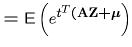
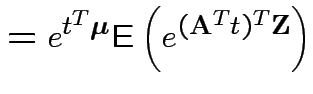
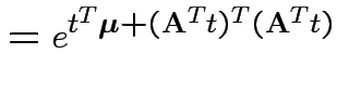
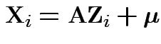
has a multivariate normal distribution if it
has the same distribution as
 for some
 , some
 matrix of constants
 ![]() and
and
 .
.
 ,
, ![]() singular:
singular: ![]() does not have a density.
does not have a density.
![]() invertible: derive multivariate normal density
by change of variables:
invertible: derive multivariate normal density
by change of variables:
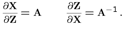
 |
 |
|
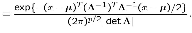 |
 density. Note density is
the same for all .
density. Note density is
the same for all .
For which
![]() ,
,
![]() is this a density?
is this a density?
Any
![]() but if
but if
 then
then
 |
 |
|
 |
||
 |
 . Inequality strict except for
  which
is equivalent to
which
is equivalent to
Conversely, if
![]() is a positive definite symmetric matrix
then there is a square invertible matrix
is a positive definite symmetric matrix
then there is a square invertible matrix ![]() such that
such that
![]() so that
there is a
distribution. (
so that
there is a
distribution. (![]() can be found
via the Cholesky decomposition, e.g.)
can be found
via the Cholesky decomposition, e.g.)
When ![]() is singular
is singular ![]() will not
have a density:
will not
have a density: ![]() such that
such that
 ;
; ![]() is confined to a hyperplane.
is confined to a hyperplane.
Still true: distribution of ![]() depends only on
depends only on
![]() : if
: if
![]() then
and
then
and
 have the same distribution.
Defn: If
has density ![]() then
then
FACT: if  for a smooth
 ![]() (mapping
(mapping
![]() )
)
 |
 |
|
 |
||
 |
 .
.
Linearity:
 for real
 ![]() and
and ![]() .
.
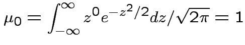
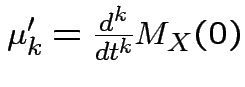
Defn: The
![]() moment (about the origin) of a real
rv
moment (about the origin) of a real
rv ![]() is
is
 (provided it exists).
We generally use
(provided it exists).
We generally use
![]() for
for
 .
.
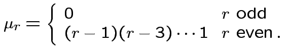
Defn: The
![]() central moment is
central moment is
![$\displaystyle \mu_r = {\rm E}[(X-\mu)^r]
$](img370.gif)
 the variance.
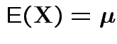
Defn: For an
![]() valued random vector
valued random vector ![]()
 (provided all entries exist).
Fact: same idea used for random matrices.
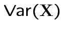
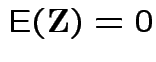
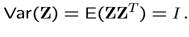
Defn: The (
 ) variance covariance matrix of
 ![]() is
is
![$\displaystyle {\rm Var}({\bf X}) = {\rm E}\left[ ({\bf X}-\boldsymbol{\mu})({\bf X}-\boldsymbol{\mu})^T \right]
$](img376.gif)
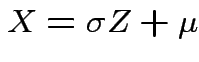
Example moments: If
 then
then
 |
 |
|
 |
||
 |
 |
 |
|
 |
||
 |
 . Remembering that
 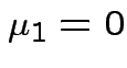 and
and
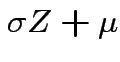
If now
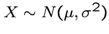 , that is,
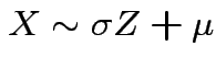 ,
then
,
then
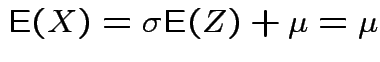 and
and
![$\displaystyle \mu_r(X) = {\rm E}[(X-\mu)^r] = \sigma^r {\rm E}(Z^r)
$](img395.gif)
 for
the distribution of
for
the distribution of
 is justified;
Similarly for
 we have
 with
with
 and
and
 |
 |
|
 |
||
 |
||
 |
 and
and
Theorem: If
 are independent and each
 ![]() is
integrable then
is
integrable then
 is integrable and
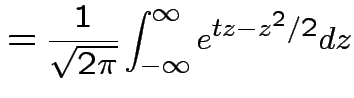
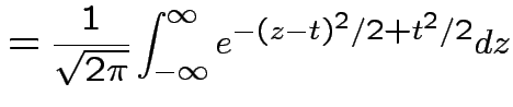
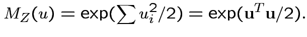
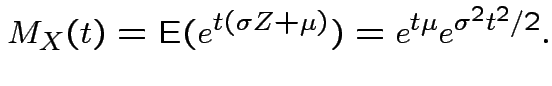
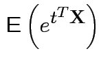
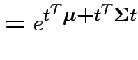
Defn: The moment generating function of a real valued ![]() is
is

Defn: The moment generating function of
is
![$\displaystyle M_{\bf X}(u) = {\rm E}[e^{u^T{\bf X}}]
$](img414.gif)
Example: If
then
 |
 |
|
 |
||
 |
||
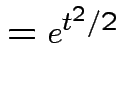 |
Theorem: ( ) If
) If ![]() is finite for all
is finite for all ![]() in a neighbourhood of
in a neighbourhood of ![]() then
then
 .
.
Note: ![]() means has continuous derivatives of all orders. Analytic
means has convergent power series expansion in neighbourhood of each
means has continuous derivatives of all orders. Analytic
means has convergent power series expansion in neighbourhood of each
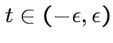 .
.
The proof, and many other facts about mgfs, rely on techniques of complex variables.
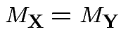
Theorem: Suppose ![]() and
and ![]() are
are
![]() valued random
vectors such that
valued random
vectors such that
The proof relies on techniques of complex variables.
If
are independent and
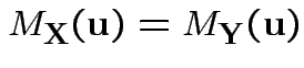
 then
mgf of
then
mgf of ![]() is product mgfs
of individual
is product mgfs
of individual ![]() :
:
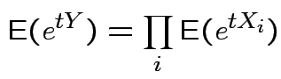
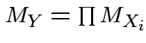 . (Also for multivariate
Example: If
 are independent
  then
then
 |
 |
|
 |
||
 |
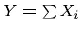
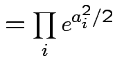
Conclusion: If
 then
then
Example: If
then
 and
and
Theorem: Suppose
 and
and
 where
where
 and
and
 . Then
![]() and
and ![]() have the same distribution if and only iff the
following two conditions hold:
have the same distribution if and only iff the
following two conditions hold:
 .
.
 .
.
Alternatively: if ![]() ,
, ![]() each MVN
then
each MVN
then
 and
and
 imply that
 ![]() and
and ![]() have
the same distribution.
have
the same distribution.
Proof: If 1 and 2 hold the mgf of ![]() is
is
 |
 |
|
 |
||
 |
||
 |
 . Conversely if
Thus mgf is determined by
![]() and
and
![]() .
.
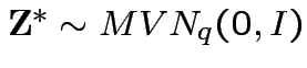
Theorem: If
 then
there is
then
there is ![]() a
matrix such that
a
matrix such that ![]() has same distribution
as
for
.
has same distribution
as
for
.
We may assume that ![]() is symmetric and non-negative definite,
or that
is symmetric and non-negative definite,
or that ![]() is upper triangular, or that
is upper triangular, or that ![]() is lower triangular.
is lower triangular.
Proof: Pick any ![]() such that
such that
![]() such as
such as
![]() from the spectral decomposition. Then
from the spectral decomposition. Then
 .
.
From the symmetric square root can produce an upper triangular square root by
the Gram Schmidt process: if ![]() has rows
has rows
 then let
 ![]() be
be
 . Choose
  proportional to
 where
where
 so that has unit length. Continue in this
way; you automatically get
so that has unit length. Continue in this
way; you automatically get
 if
if  . If
. If ![]() has
columns
has
columns
 then
then ![]() is orthogonal and
is orthogonal and
![]() is an
upper triangular square root of
is an
upper triangular square root of
![]() .
.
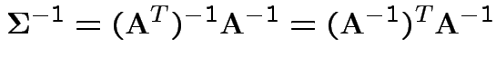
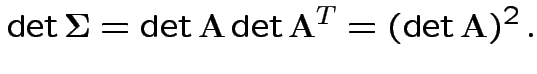
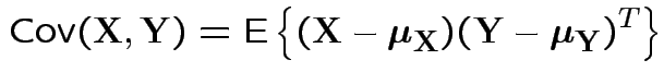
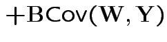
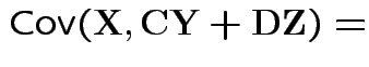
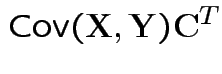
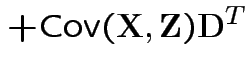
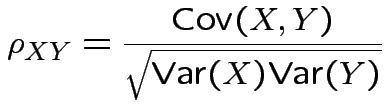
Defn: The covariance between ![]() and
and ![]() is
is
Properties:
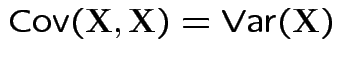 .
.
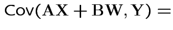 |
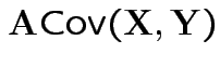 |
|
 |
 |
 |
|
 |
Properties of the ![]() distribution
distribution
1: All margins are multivariate normal: if
![$\displaystyle {\bf X}= \left[\begin{array}{c} {\bf X}_1\\ {\bf X}_2\end{array} \right]
$](img481.gif)
![$\displaystyle \mu = \left[\begin{array}{c} \mu_1\\ \mu_2\end{array} \right]
$](img482.gif)
![$\displaystyle \boldsymbol{\Sigma} = \left[\begin{array}{cc} \boldsymbol{\Sigma}...
...}
\\
\boldsymbol{\Sigma}_{21} & \boldsymbol{\Sigma}_{22} \end{array} \right]
$](img483.gif)
 .
.
2:
 : affine
transformation of MVN is normal.
: affine
transformation of MVN is normal.
3: If
 and
and  are independent.
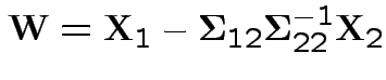
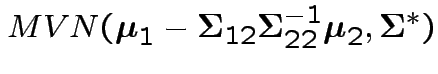
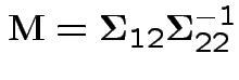
4: All conditionals are normal: the conditional distribution of
given
 is
is
 Proof of ( 1): If
 then
then
![$\displaystyle {\bf X}_1 = \left[ I \vert {\bf0}\right] {\bf X}
$](img492.gif)
So
![$\displaystyle {\bf X}_1 = \left( \left[ I \vert {\bf0}\right]{\bf A}\right) {\bf Z}+ \left[ I \vert {\bf0}\right]
\boldsymbol{\mu}
$](img493.gif)
Compute mean and variance to check rest.
Proof of ( 2): If
then
Proof of ( 3): If
![$\displaystyle {\bf u} = \left[\begin{array}{c}{\bf u}_1 \\ {\bf u}_2\end{array}\right]
$](img495.gif)
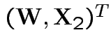
Proof of ( 4): first case: assume
 has an inverse.
Define
![$\displaystyle \left[\begin{array}{c}
{\bf W}\\ {\bf X}_2\end{array}\right]
=
\...
...array}\right]
\left[\begin{array}{c}
{\bf X}_1 \\ {\bf X}_2\end{array}\right]
$](img499.gif)
 is
is
 where
where
![$\displaystyle \boldsymbol\Sigma^* = \left[\begin{array}{cc}
\boldsymbol\Sigma_{...
...mbol\Sigma_{21} & {\bf0} \\
{\bf0}& \boldsymbol\Sigma_{22}\end{array}\right]
$](img502.gif)
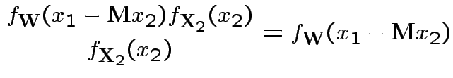
Now joint density of ![]() and
and ![]() factors
factors
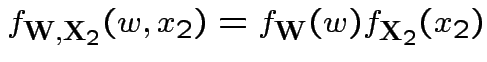

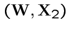 to
to
 and
and
 given
is
given
is
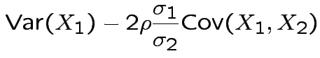
Specialization to bivariate case:
Write
![$\displaystyle \boldsymbol\Sigma = \left[\begin{array}{cc} \sigma_1^2 & \rho\sigma_1\sigma_2
\\
\rho\sigma_1\sigma_2
& \sigma_2^2\end{array}\right]
$](img512.gif)
Then
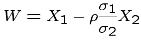
 . The marginal distribution of
 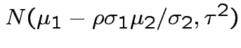 where
where
 |
 |
|
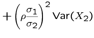 |
This simplifies to

More generally: any ![]() and
and ![]() :
:
| 0 | 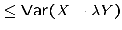 |
|
 |
is scalar but is vector.
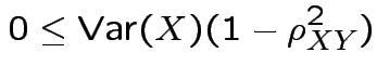
Defn: Multiple correlation between and
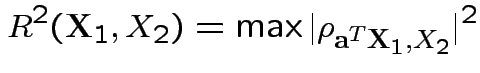
 .
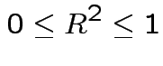
.
Thus: maximize
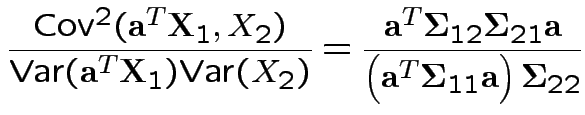
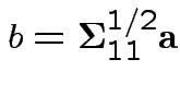 . For
. For
 invertible problem is
equivalent to maximizing
invertible problem is
equivalent to maximizing
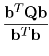
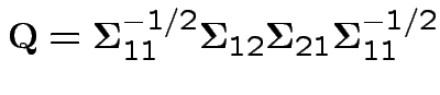
Note
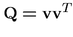
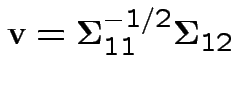
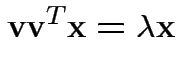
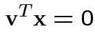 or
or 
Summary: maximum squared correlation is
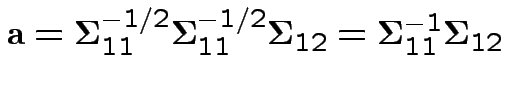
Notice: since ![]() is squared correlation between two scalars
(
is squared correlation between two scalars
(
 and ) we have
 is linear combination of .
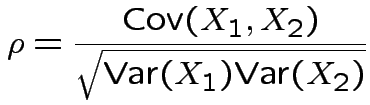
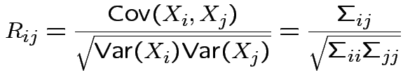
Correlation matrices, partial correlations:
Correlation between two scalars ![]() and
and ![]() is
is
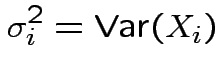
If ![]() has variance
has variance
![]() then the correlation matrix of
then the correlation matrix of ![]() is
is
 with entries
If
 are MVN with the usual partitioned variance covariance matrix
then the conditional variance of given is
are MVN with the usual partitioned variance covariance matrix
then the conditional variance of given is
From this define partial correlation matrix
Note: these are used even when
are NOT MVN
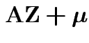
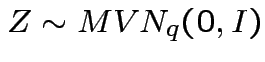
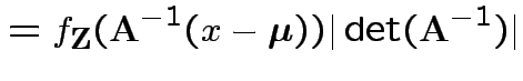
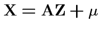
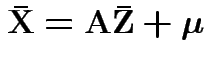
Given data ![]() with model
with model
 :
:
Definition: The likelihood function is map ![]() : domain
: domain
![]() , values given by
, values given by
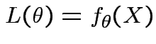
Key Point: think about how the density depends on ![]() not
about how it depends on
not
about how it depends on ![]() .
.
Notice: ![]() , observed value of the
data, has been plugged into the formula for density.
, observed value of the
data, has been plugged into the formula for density.
We use likelihood for most inference problems:
 which lies in
  over
over
 if such a
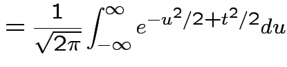
 of
of
 . We use
 where
where
 in
in
 where
where
 . We base our
decision
on the likelihood ratio
. We base our
decision
on the likelihood ratio
Maximum Likelihood Estimation
To find MLE maximize ![]() .
.
Typical function maximization problem:
Set gradient of ![]() equal to 0
equal to 0
Check root is maximum, not minimum or saddle point.
Often ![]() is product of
is product of ![]() terms (given
terms (given ![]() independent observations).
independent observations).
Much easier to work with logarithm
of ![]() : log of product is sum and logarithm is monotone
increasing.
: log of product is sum and logarithm is monotone
increasing.
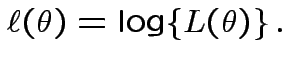
Definition: The Log Likelihood function is
Simplest problem: collect replicate measurements
 from single population.
Model: ![]() are iid
are iid
 .
.
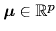
Parameters (![]() ):
):
 .
Parameter space:
.
Parameter space:
 and
and
![]() is some positive definite matrix.
is some positive definite matrix.
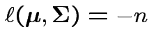
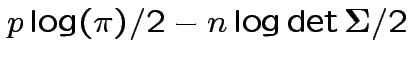
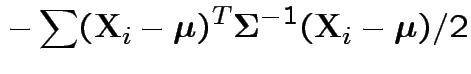
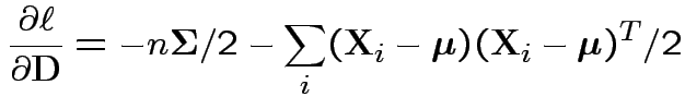
Log likelihood is
 |
 |
|
 |
 |
 |
|
 |
 .
Second derivative wrt
.
Second derivative wrt
Fact: if second derivative matrix is negative definite everywhere then function is concave; no more than 1 critical point.
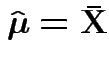
Summary: ![]() is maximized at
is maximized at
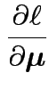
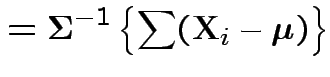
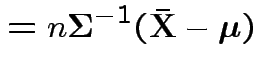
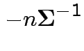
More difficult: differentiate ![]() wrt
wrt
![]() .
.
Somewhat simpler: set
![]()
First derivative wrt ![]() is matrix with entries
is matrix with entries
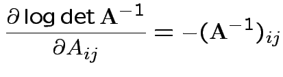
Need: derivative of two functions:
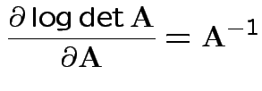
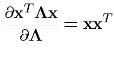
Fact:
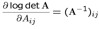
![]() th entry of
th entry of
![]() is
is
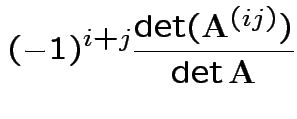
Fact:
 ; expansion
by minors.
; expansion
by minors.
Conclusion
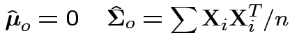
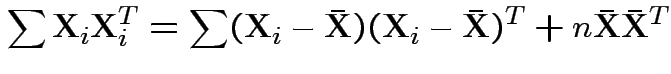
Set = 0 and find only critical point is
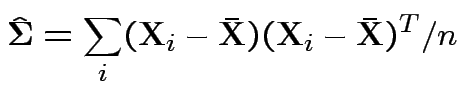
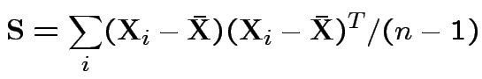
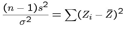
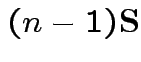
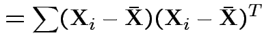
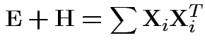
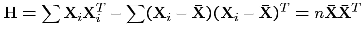
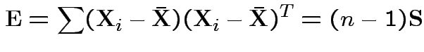
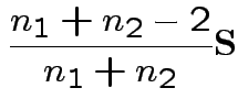
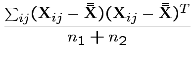
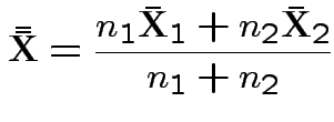
Usual sample covariance matrix is
Properties of MLEs:
1)
2)
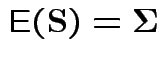 .
.
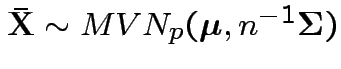
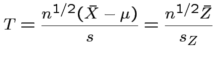
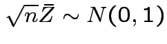
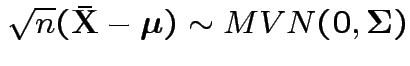
Distribution of ![]() ? Joint distribution of
? Joint distribution of
![]() and
and ![]() ?
?
Theorem:
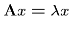
Suppose
 are independent
random
variables.
Then
are independent
random
variables.
Then
 .
.
 .
.
 .
.
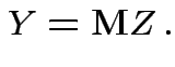
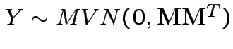
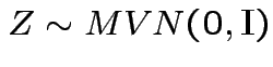
Proof: Let
 .
.
Then
are
independent .
So
 is multivariate
standard normal.
is multivariate
standard normal.
Note that
 and
and
 Thus
Thus
 .
.
So: reduced to  and
and ![]() .
.
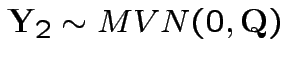
Step 1: Define

 .) Now
![$\displaystyle Y =\left[\begin{array}{cccc}
\frac{1}{\sqrt{n}} &
\frac{1}{\sqrt{...
...]
\left[\begin{array}{c}
Z_1 \\
Z_2 \\
\vdots
\\
Z_n
\end{array}\right]
$](img628.gif)
 so we need
to compute
so we need
to compute
 |
![$\displaystyle = \left[\begin{array}{c\vert cccc} 1 & 0 & 0 & \cdots & 0 \\ \hli...
...ots & -\frac{1}{n} \\ 0 & \vdots & \cdots & & 1-\frac{1}{n} \end{array} \right]$](img634.gif) |
|
![$\displaystyle = \left[\begin{array}{c\vert c} 1 & 0 \\ \hline \\ 0 & {\bf Q} \end{array} \right] \,.$](img635.gif) |
Put
 . Since
 are independent and each is normal.
Thus
 is independent of
 .
.
Since ![]() is a function of
we see that
and
is a function of
we see that
and
![]() are independent.
are independent.
Also, see
 .
.
First 2 parts done.
Consider
 .
Note that
.
Note that
 .
.
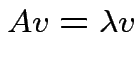
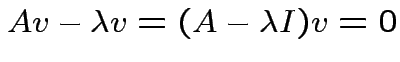
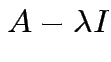
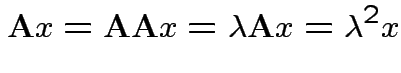
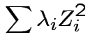
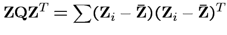
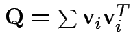
Now: distribution of quadratic forms:
Suppose
 and
and ![]() is symmetric.
Put
is symmetric.
Put
![]() for
for ![]() diagonal,
diagonal, ![]() orthogonal.
orthogonal.
Then
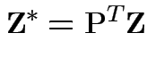
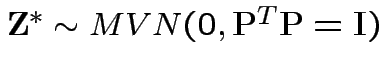 is standard multivariate normal.
So:
![]() has same distribution as
has same distribution as

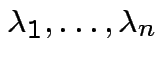 are eigenvalues of
Special case: if all ![]() are either 0 or 1 then
are either 0 or 1 then
![]() has a chi-squared distribution with df
= number of
has a chi-squared distribution with df
= number of ![]() equal to 1.
equal to 1.
When are eigenvalues all 1 or 0?
Answer: if and only if ![]() is idempotent.
is idempotent.
1) If ![]() idempotent and
idempotent and
 is an eigenpair
the
is an eigenpair
the

2) Conversely if all eigenvalues of ![]() are 0 or 1 then
are 0 or 1 then
![]() has 1s and 0s on diagonal so
has 1s and 0s on diagonal so
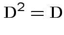
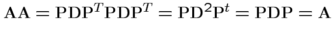
 . Then
Since
![]() it has the law
it has the law
So eigenvalues are those of
![]() and
and
![]() is
is
![]() iff
iff
![]() is idempotent and
is idempotent and
 .
.
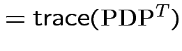
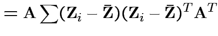
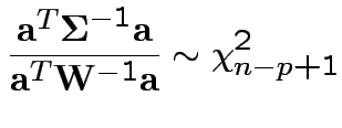
Our case:
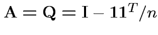 .
Check
.
Check
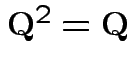 .
How many degrees of freedom:
.
How many degrees of freedom:
 .
.
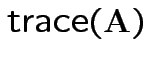
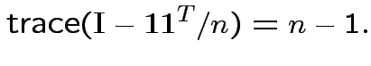
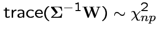
Defn: The trace of a square matrix ![]() is
is

Property:
 .
.
So:
 |
 |
|
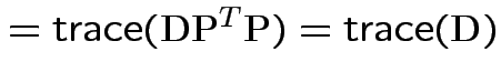 |
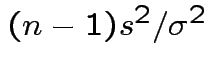
Conclusion: df for
 is
is
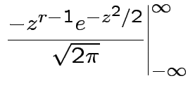
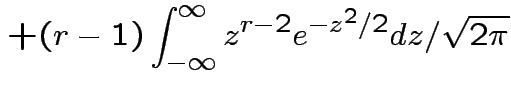
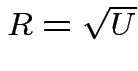
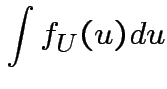
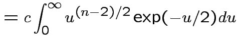
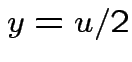
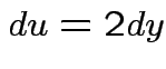
Derivation of the ![]() density:
density:
Suppose
 independent . Define
![]() distribution to be that of
distribution to be that of
 .
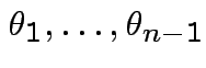
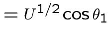
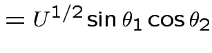
Define angles
.
Define angles
 by
by
 |
||
 |
||
 |
||
 |
 |
|
 |
 .
.
Matrix of partial derivatives is
![$\displaystyle \left[\begin{array}{ccc}
\frac{\cos\theta_1}{2R}
&
-R \sin\theta_...
...R \cos\theta_1\sin\theta_2
&
R \sin\theta_1\cos\theta_2
\end{array}\right] \,.
$](img701.gif)
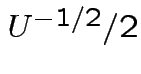 while
every other entry has a factor
while
every other entry has a factor
FACT: multiplying a column in a matrix by ![]() multiplies
the determinant by
multiplies
the determinant by ![]() .
.
SO: Jacobian of transformation is
Thus joint density
of
 is
is
 dimensional
multiple integral
dimensional
multiple integral
 .
.
Answer has the form
Evaluate ![]() by making
by making
 |
 |
|
 |
 ,
,  to see that
 |
 |
|
|
Fourth part: consequence of
first 3 parts and def'n of ![]() distribution.
distribution.
Defn:
 if
if ![]() has same distribution
as
has same distribution
as
 ,
,
 and
and  independent.
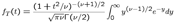
Derive density of ![]() in this definition:
in this definition:
 |
 |
|
 |
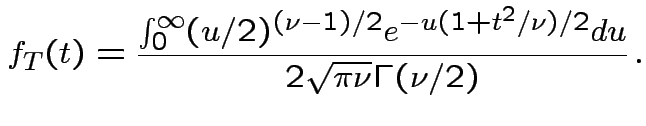
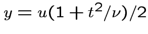 , to get
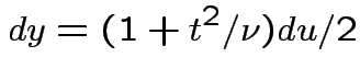
![$\displaystyle (u/2)^{(\nu-1)/2}= [y/(1+t^2/\nu)]^{(\nu-1)/2}$](img737.gif)
Theorem:
Suppose
are independent
 random
variables.
Then
random
variables.
Then
 .
.
 .
.
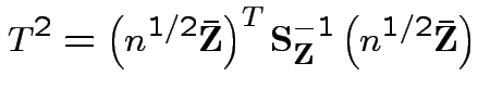
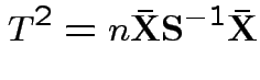
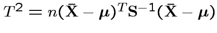 is Hotelling's
 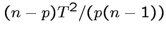 has an
 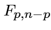 distribution.
Proof: Let
 where
where
![]() and
and
 are
independent
are
independent
 .
.
So
 .
.
Note that
 and
and
 |
 |
|
 |

Consequences. In 1, 2 and 4: can assume
 and
and
![]() . In 3 can take
.
Step 1: Do general
. In 3 can take
.
Step 1: Do general
![]() . Define
. Define
 .) Clearly
 Compute variance covariance matrix
![$\displaystyle \left[\begin{array}{cc}
{\bf I}_{p\times p} & 0 \\
0 & {\bf Q}^*
\end{array}\right]
$](img763.gif)
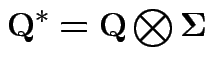
 has a pattern. It is a
patterned matrix with entry
has a pattern. It is a
patterned matrix with entry 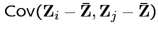 |
 |
|
 |
Defn: If ![]() is
and
is
and ![]() is
is
 then
then
 is the
 matrix with the pattern
![$\displaystyle \left[\begin{array}{cccc}
{\bf A}_{11}{\bf B}& {\bf A}_{12}{\bf B...
...{\bf B}& {\bf A}_{p2} {\bf B}& \cdots & {\bf A}_{pq}{\bf B}
\end{array}\right]
$](img773.gif)
Conclusions so far:
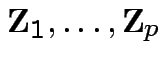
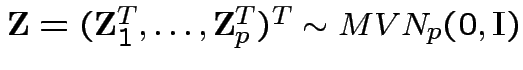
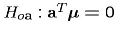
1)
![]() and
and ![]() are independent.
are independent.
2)
Next: Wishart law.
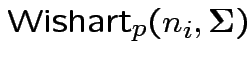
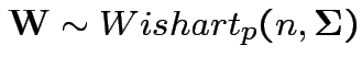
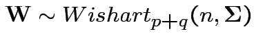
Defn: The
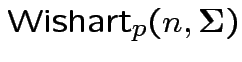 distribution is
the distribution of
distribution is
the distribution of
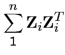
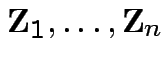 are iid
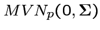 .
.
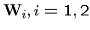
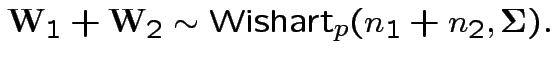
Properties of Wishart.
1) If
![]() then
then
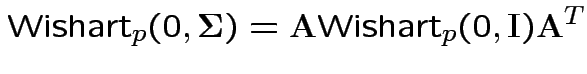
2) if
 independent
 then
then
Proof of part 3: rewrite
 .
Put
as
cols in matrix
.
Put
as
cols in matrix  . Then
check that
. Then
check that
 for orthogonal
unit vectors
for orthogonal
unit vectors
 .
Define
.
Define
 .
Then check that
.
Then check that
Uses further props of Wishart distribution.
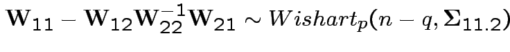
3: If
 and
and
 then
then
4: If
and  then
then
5: If
then
6: If
 is partitioned
into components then
is partitioned
into components then
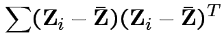
Given data
iid
 test
test
Example: no realistic ones. This hypothesis is not intrinsically useful. However: other tests can sometimes be reduced to it.
Example: Ten water samples split in half. One half of each
to each of two labs. Measure biological oxygen demand (BOD) and
suspended solids (SS). For sample ![]() let
let  be BOD for lab A,
 be SS for lab A,
  be BOD for lab B and
  be
SS for lab B. Question: are labs measuring the same thing? Is there
bias in one or the other?
be
SS for lab B. Question: are labs measuring the same thing? Is there
bias in one or the other?
Notation ![]() is vector of 4 measurements on sample
is vector of 4 measurements on sample ![]() .
.
Data:
| Lab A | Lab B | |||
| Sample | BOD | SS | BOD | SS |
| 1 | 6 | 27 | 25 | 15 |
| 2 | 6 | 23 | 28 | 13 |
| 3 | 18 | 64 | 36 | 22 |
| 4 | 8 | 44 | 35 | 29 |
| 5 | 11 | 30 | 15 | 31 |
| 6 | 34 | 75 | 44 | 64 |
| 7 | 28 | 26 | 42 | 30 |
| 8 | 71 | 124 | 54 | 64 |
| 9 | 43 | 54 | 34 | 56 |
| 10 | 33 | 30 | 29 | 20 |
| 11 | 20 | 14 | 39 | 21 |
Model:
 are iid
 .
.
Multivariate problem because: not able to assume independence between any two measurements on same sample.
Potential sub-model: each measurement is
true mmnt + lab bias + mmnt error.
Model for measurement error vector
![]() is multivariate normal mean 0 and diagonal covariance
matrix
is multivariate normal mean 0 and diagonal covariance
matrix
 .
.
Lab bias is unknown vector
![]() .
.
True measurement should be same for both labs so has form
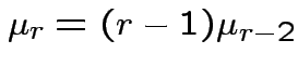
![$\displaystyle [Y_{i1},Y_{i2},Y_{i1},Y_{i2}]
$](img815.gif)
 are iid bivariate normal with unknown
means
are iid bivariate normal with unknown
means
 and unknown
 variance
covariance
variance
covariance
 .
.
This would give structured model
![$\displaystyle {\bf C}= \left[\begin{array}{cc} 1 & 0 \\ 0 & 1 \\ 1 & 0 \\ 0 &
1\end{array}\right]
$](img821.gif)
This model has variance covariance matrix
 and 3 for the entries in
.
and 3 for the entries in
.
We skip this model and let
 be unrestricted.
Question of interest:
 and
and 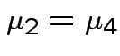
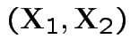
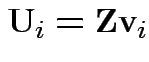
Reduction: partition ![]() as
as
![$\displaystyle \left[\begin{array}{c} {\bf U}_i \\ {\bf V}_i \end{array}\right]
$](img826.gif)
Define
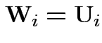 . Then our model makes
  iid
iid
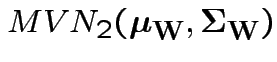 .
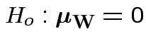
Our hypothesis is
.
Our hypothesis is
Carrying out our test in SPlus:
Working on CSS unix workstation:
Start SPlus then read in, print out data:
[61]ehlehl% mkdir .Data
[62]ehlehl% Splus
S-PLUS : Copyright (c) 1988, 1996 MathSoft, Inc.
S : Copyright AT&T.
Version 3.4 Release 1 for Sun SPARC, SunOS 5.3 : 1996
Working data will be in .Data
> # Read in and print out data
> eff <- read.table("effluent.dat",header=T)
> eff
   BODLabA SSLabA BODLabB SSLabB
 1       6     27      25     15
 2       6     23      28     13
 3      18     64      36     22
 4       8     44      35     29
 5      11     30      15     31
 6      34     75      44     64
 7      28     26      42     30
 8      71    124      54     64
 9      43     54      34     56
10      33     30      29     20
11      20     14      39     21
Do some graphical preliminary analysis.
Look for non-normality, non-linearity, outliers.
Make plots on screen or saved in file.
> # Make pairwise scatterplots on screen using
> # motif graphics device and then in a postscript
> # file.
> motif()
> pairs(eff)
> postscript("pairs.ps",horizontal=F,
+   height=6,width=6)
> pairs(eff)
> dev.off()
Generated postscript file "pairs.ps".
 motif
     2
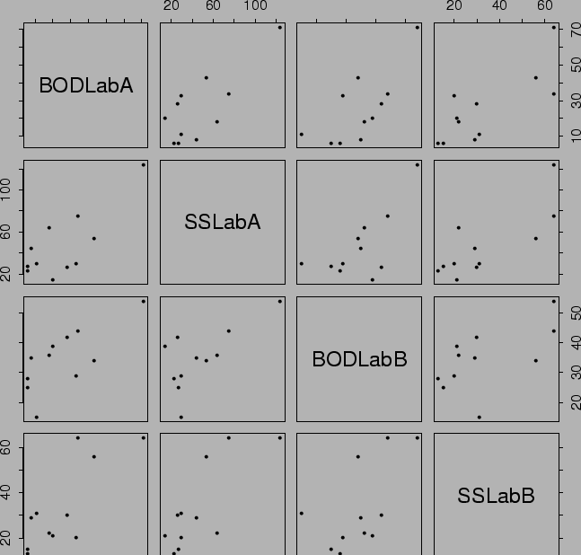
> cor(eff)
          BODLabA    SSLabA   BODLabB    SSLabB
BODLabA 0.9999999 0.7807413 0.7228161 0.7886035
 SSLabA 0.7807413 1.0000000 0.6771183 0.7896656
BODLabB 0.7228161 0.6771183 1.0000001 0.6038079
 SSLabB 0.7886035 0.7896656 0.6038079 1.0000001
Notice high correlations.
Mostly caused by variation in true levels from sample to sample.
Get partial correlations.
Adjust for overall BOD and SS content of sample.
> aug <- cbind(eff,(eff[,1]+eff[,3])/2,
+                  (eff[,2]+eff[,4])/2)
> aug
   BODLabA SSLabA BODLabB SSLabB   X2   X3
 1       6     27      25     15 15.5 21.0
 2       6     23      28     13 17.0 18.0
 3      18     64      36     22 27.0 43.0
 4       8     44      35     29 21.5 36.5
 5      11     30      15     31 13.0 30.5
 6      34     75      44     64 39.0 69.5
 7      28     26      42     30 35.0 28.0
 8      71    124      54     64 62.5 94.0
 9      43     54      34     56 38.5 55.0
10      33     30      29     20 31.0 25.0
11      20     14      39     21 29.5 17.5
> bigS <- var(aug)
Now compute partial correlations for first four variables given means of BOD and SS:
> S11 <- bigS[1:4,1:4]
> S12 <- bigS[1:4,5:6]
> S21 <- bigS[5:6,1:4]
> S22 <- bigS[5:6,5:6]
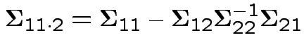
> S11dot2 <- S11 - S12 %*% solve(S22,S21)
> S11dot2
BODLabA SSLabA BODLabB SSLabB
BODLabA 24.804665 -7.418491 -24.804665 7.418491
SSLabA -7.418491 59.142084 7.418491 -59.142084
BODLabB -24.804665 7.418491 24.804665 -7.418491
SSLabB 7.418491 -59.142084 -7.418491 59.142084
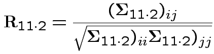
> S11dot2SD <- diag(sqrt(diag(S11dot2)))
> S11dot2SD
[,1] [,2] [,3] [,4]
[1,] 4.980428 0.000000 0.000000 0.000000
[2,] 0.000000 7.690389 0.000000 0.000000
[3,] 0.000000 0.000000 4.980428 0.000000
[4,] 0.000000 0.000000 0.000000 7.690389
> R11dot2 <- solve(S11dot2SD)%*%
+ S11dot2%*%solve(S11dot2SD)
> R11dot2
[,1] [,2] [,3] [,4]
[1,] 1.000000 -0.193687 -1.000000 0.193687
[2,] -0.193687 1.000000 0.193687 -1.000000
[3,] -1.000000 0.193687 1.000000 -0.193687
[4,] 0.193687 -1.000000 -0.193687 1.000000
Notice little residual correlation.
Carry out Hotelling's  .
.
> w <- eff[,1:2]-eff[3:4]
> dimnames(w)<-list(NULL,c("BODdiff","SSdiff"))
> w
      BODdiff SSdiff
 [1,]     -19     12
 [2,]     -22     10
  etc
 [8,]      17     60
  etc
> Sw <- var(w)
> cor(w)
          BODdiff    SSdiff
BODdiff 1.0000001 0.3057682
 SSdiff 0.3057682 1.0000000
> mw <- apply(w,2,mean)
> mw
   BODdiff   SSdiff
 -9.363636 13.27273
> Tsq <- 11*mw%*%solve(Sw,mw)
> Tsq
         [,1]
[1,] 13.63931
> FfromTsq <- (11-2)*Tsq/(2*(11-1))
> FfromTsq
        [,1]
[1,] 6.13769
> 1-pf(FfromTsq,2,9)
[1] 0.02082779
Conclusion: Pretty clear evidence of difference in mean level between
labs.
Which measurement causes the difference?
> TBOD <- sqrt(11)*mw[1]/sqrt(Sw[1,1])
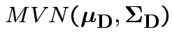
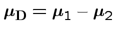
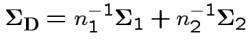
> TBOD
BODdiff
-2.200071
> 2*pt(TBOD,1)
BODdiff
0.2715917
> 2*pt(TBOD,10)
BODdiff
0.05243474
> TSS <- sqrt(11)*mw[2]/sqrt(Sw[2,2])
> TSS
SSdiff
2.15153
> 2*pt(-TSS,10)
SSdiff
0.05691733
> postscript("differences.ps",
+ horizontal=F,height=6,width=6)
> plot(w)
> abline(h=0)
> abline(v=0)
> dev.off()
Conclusion? Neither? Not a problem - summarizes evidence!
Problem: several tests at level 0.05 on same data. Simultaneous or Multiple comparisons.
 by computing
 and then testing
 using Hotelling's
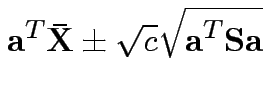
Confidence interval for
 :
:
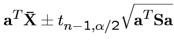
Give coverage intervals for 6 parameters of interest: 4 entries in
![]() and
and
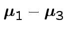 and
and
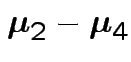
|
|
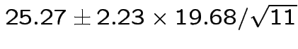 |
|
|
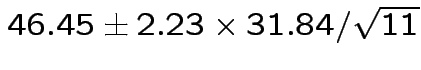 |
|
|
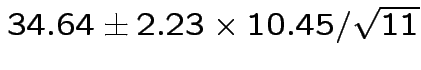 |
|
|
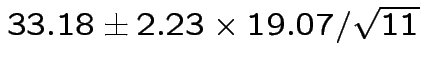 |
|
|
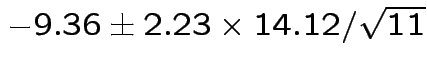 |
|
|
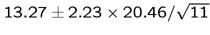 |
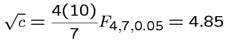
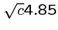
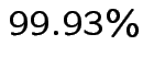
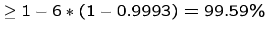
Problem: each confidence interval has 5% error rate. Pick out last interval (on basis of looking most interesting) and ask about error rate?
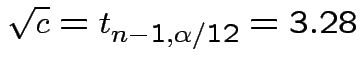
Solution: adjust 2.23, ![]() multiplier to get
multiplier to get
 all intervals cover truth
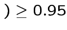
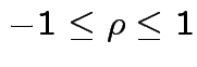
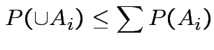
Based on inequality:
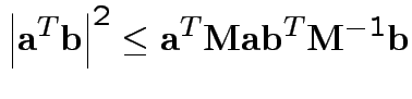
Proof by Cauchy Schwarz:
inner product of vectors
![]() and
and
![]() .
.
Put
 and
and
![]() to get
to get

 .
.
In fact the probability of this happening is exactly equal to because for
each data set the supremum of
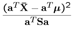
Our case
Coverage probability of single interval using
 ?
From
?
From ![]() distribution:
distribution:
Probability all 6 intervals would cover using
?
Use Bonferroni inequality:
Usually just use
General Bonferroni strategy. If we want intervals for
 get interval for
 ![]() at
level
at
level
 . Simultaneous coverage probability is
at least . Notice that Bonferroni narrower in
our example unless
. Simultaneous coverage probability is
at least . Notice that Bonferroni narrower in
our example unless
![]() giving
giving  .
.
Motivations for ![]() :
:
1: Hypothesis
 is true iff all
hypotheses
is true iff all
hypotheses
 are true.
Natural test for
are true.
Natural test for
 rejects if
Fact:
2: likelihood ratio method.
Compute
 .
.
In our case to test
find

Now write
Again conclude: likelihood ratio test rejects for 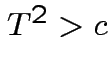 where
where ![]() chosen to make level
chosen to make level ![]() .
.
3: compare estimates of
![]() .
.
In univariate regression ![]() tests to compare a restricted model with a full model
have form
tests to compare a restricted model with a full model
have form
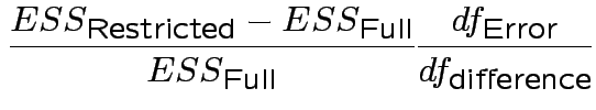
 .
.
Here: substitute matrices.
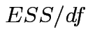
Analogue of ESS for full model:
Analogue of ESS for reduced model:
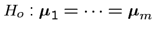
In 1 sample example:
Test of
based on comparing
To make comparison. If null true

Measures of size based on eigenvalues of
Suggested size measures for
 :
:
 (= sum of eigenvalues).
 (= product of eigenvalues).
.
For our matrix: eigenvalues all 0 except for one.
(So really-matrix not close to ![]() .)
.)
Largest eigenvalue is
But: see two sample problem for precise tests based on suggestions.
 .
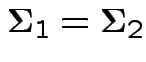
Model
.
Model
 , independent.
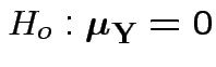
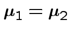
Test
 .
.
Case 1: for motivation only.
![]() known
known  .
.
Natural test statistic: based on
 where
where
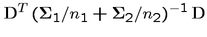
If
![]() not known must estimate. No universally
agreed best procedure (even for -- called Behrens-Fisher problem).
not known must estimate. No universally
agreed best procedure (even for -- called Behrens-Fisher problem).
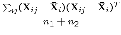
Usually: assume
 .
.
If so: MLE of
![]() is
is
![]() and of
and of
![]() is
is
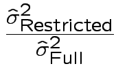
Possible test developments:
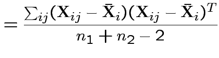
1) By analogy with 1 sample:
 Pooled
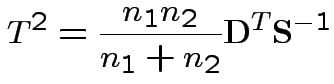
2) Union-intersection: test of
 based on
Get
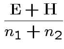
3) Likelihood ratio: the MLE of
![]() for the unrestricted model
is
for the unrestricted model
is
 the mle of
This simplifies to
 Full
Full Restricted
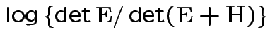
If ![]() are the eigenvalues of
are the eigenvalues of
![]() then
then
Two sample analysis in SAS on css network
    data long;
    infile 'tab57sh';
    input group a b c;
run;
proc print;
run;
proc glm;
    class group;
    model a b c = group;
    manova h=group / printh printe;
run;
Notes:
1) First 4 lines form DATA step:
a) creates data set named long by reading in 4 columns of data from file named tab57sh stored in same directory as I was in when I typed sas.
b) Calls variables group (=1 or 2 as label for the two groups) and a, b, c which are names for the 3 test scores for each subject.
2) Next two lines: print out data: result is (slightly edited)
    Obs    group     a     b     c
      1      1      19    20    18
      2      1      20    21    19
      3      1      19    22    22
     etc till
     11      2      15    17    15
     12      2      13    14    14
     13      2      14    16    13
3) Then use proc glm to do analysis:
a) class group declares that the variable group defines levels of a categorical variable.
b) model statement says to regress the variables a, b, c on variable group.
c) manova statement says to do both 3 univariate regressions
and a mulivariate regression and to print out the ![]() and
and ![]() matrices where
matrices where ![]() is the matrix corresponding to the presence
of the factor group in the model.
is the matrix corresponding to the presence
of the factor group in the model.
Output of MANOVA: First univariate results
    The GLM Procedure
 Class Level Information
        Class         Levels    Values
        group              2    1 2
 Number of observations    13
Dependent Variable: a
                Sum of
Source    DF   Squares  Mean Square F Value Pr > F
Model      1  54.276923  54.276923   19.38 0.0011
Error     11  30.800000   2.800000
Corrd Tot 12  85.076923
R-Square   Coeff Var      Root MSE        a Mean
0.637975    10.21275      1.673320      16.38462
Source    DF  Type ISS  Mean Square F Value Pr > F
group      1  54.276923  54.276923   19.38 0.0011
Source    DF  TypeIIISS Mean Square F Value Pr > F
group      1  54.276923  54.276923   19.38 0.0011

Dependent Variable: b
                Sum of
Source    DF   Squares  Mean Square F Value Pr > F
Model      1  70.892308  70.892308  34.20 0.0001
Error     11  22.800000   2.072727
Corrd Tot 12  93.692308

Dependent Variable: c
                Sum of
Source    DF   Squares Mean Square F Value Pr > F
Model      1   94.77692  94.77692   39.64 <.0001
Error     11   26.30000   2.39090
Corrd Tot 12  121.07692
The matrices
  E = Error SSCP Matrix
   a     b     c
a 30.8  12.2  10.2
b 12.2  22.8   3.8
c 10.2   3.8  26.3
Partial Correlation Coefficients from
    the Error SSCP Matrix / Prob > |r|
DF = 11     a              b              c
a    1.000000       0.460381       0.358383
                      0.1320         0.2527
b    0.460381       1.000000       0.155181
       0.1320                        0.6301
c    0.358383       0.155181       1.000000
       0.2527         0.6301
H = Type III SSCP Matrix for group
     a                 b                 c
a   54.276923077   62.030769231   71.723076923
b   62.030769231   70.892307692   81.969230769
c   71.723076923   81.969230769   94.776923077
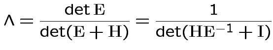
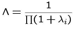
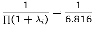
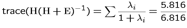
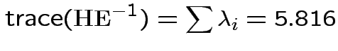
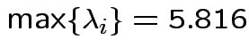
The eigenvalues of
Characteristic Roots and Vectors of: E Inverse * H
H = Type III SSCP Matrix for group
E = Error SSCP Matrix
Characteristic       Characteristic Vector V'EV=1
Root     Percent        a           b           c
5.816159 100.00  0.00403434  0.12874606 0.13332232
0.000000   0.00 -0.09464169 -0.10311602 0.16080216
0.000000   0.00 -0.19278508  0.16868694 0.00000000
MANOVA Test Criteria and Exact F Statistics
 for the Hypothesis of No Overall group Effect
H = Type III SSCP Matrix for group
E = Error SSCP Matrix
S=1    M=0.5    N=3.5
Statistic            Value   F   NumDF DenDF Pr > F
Wilks' Lambda       0.1467 17.45    3     9  0.0004
Pillai's Trace      0.8533 17.45    3     9  0.0004
Hotelling-Lawley Tr 5.8162 17.45    3     9  0.0004
Roy's Greatest Root 5.8162 17.45    3     9  0.0004
Things to notice:
Wilk's Lambda:
Data
 .
.
Model
 independent
 .
.
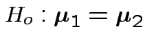
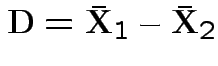
First problem of interest: test
Based on ![]() and
and ![]() . MLE of
. MLE of
![]() is
is
![]() .
.
 MLE of
 .
The data
.
The data
1 19 20 18
1 20 21 19
1 19 22 22
1 18 19 21
1 16 18 20
1 17 22 19
1 20 19 20
1 15 19 19
2 12 14 12
2 15 15 17
2 15 17 15
2 13 14 14
2 14 16 13
3 15 14 17
3 13 14 15
3 12 15 15
3 12 13 13
4  8  9 10
4 10 10 12
4 11 10 10
4 11  7 12
Code
    data three;
    infile 'tab57for3sams';
    input group a b c;
run;
proc print;
run;
proc glm;
    class group;
    model a b c = group;
    manova h=group / printh printe;
run;
    data four;
    infile 'table5.7';
    input group a b c;
run;
proc print;
run;
proc glm;
    class group;
    model a b c = group;
    manova h=group / printh printe;
run;
Pieces of output: first set of code does first 3 groups.
So: ![]() has rank 2.
has rank 2.
Characteristic Roots & Vectors of: E Inverse * H
 Characteristic     Characteristic Vector V'EV=1
      Root Percent     a        b        c
6.90568180  96.94   0.01115  0.14375 0.08795
0.21795125   3.06  -0.07763 -0.09587 0.16926
0.00000000   0.00  -0.18231  0.13542 0.02083
S=2    M=0    N=5
Statistic         Value   F   NumDF  Den DF Pr > F
Wilks'           0.1039  8.41   6      24   <.0001
Pillai's         1.0525  4.81   6      26   0.0020
Hotelling-Lawley 7.1236 13.79   6   14.353  <.0001
Roy's            6.9057 29.92   3      13   <.0001
NOTE: F Statistic for Roy's is an upper bound.
NOTE: F Statistic for Wilks'is exact.
Notice two eigenvalues not 0. Note that exact distribution
for Wilk's Lambda is available.
Now 4 groups
      Root Percent      a       b       c
15.3752900  98.30   0.01128  0.13817 0.08126
0.2307260    1.48  -0.04456 -0.09323 0.15451
0.0356937    0.23  -0.17289  0.09020 0.04777
S=3    M=-0.5    N=6.5
Statistic          Value    F    NumDF Den DF Pr > F
Wilks'         0.04790913 10.12    9   36.657 <.0001
Pillai's       1.16086747  3.58    9       51 0.0016
Hot'ng-Lawley 15.64170973 25.02    9   20.608 <.0001
Roy's         15.37528995 87.13    3       17 <.0001
NOTE: F Statistic for Roy's is an upper bound.
Test ?
Define
 Then put
 |
||
 |
||
 |
Data 
 .
.
Model: independent,
 .
.
Note: this is the fixed effects model.
Usual approach: define grand mean, main effects, interactions:
 |
||
 |
||
 |
||
 |
Test additive effects:
 for all
  .
.
Usual test based on ANOVA:
Stack observations into vector ![]() , say.
, say.
Estimate ![]() ,
, ![]() , etc by least squares.
, etc by least squares.
Form vectors with entries ![]() ,
,
![]() etc.
etc.
Write
Fact: all vectors on RHS are independent and orthogonal. So:
Our problem is like this one BUT the errors are not modeled as independent.
In the analogy:
![]() labels group.
labels group.
![]() labels the columns: ie
labels the columns: ie ![]() is a, b, c.
is a, b, c.
![]() runs from 1 to
runs from 1 to
 .
.
But
Now do analysis in SAS.
Tell SAS that the variables A, B and C are repeated measurements of the same quantity.
proc glm;
    class group;
    model a b c = group;
    repeated scale;
run;
The results are as follows:
General Linear Models Procedure
Repeated Measures Analysis of Variance
Repeated Measures Level Information
Dependent Variable  A   B    C
Level of SCALE      1   2    3

Manova Test Criteria and Exact F
   Statistics for the Hypothesis of no
   SCALE Effect
H = Type III SS&CP Matrix for SCALE
               E = Error SS&CP Matrix
S=1    M=0    N=7
Statistic
                  Value     F   NumDF DenDF Pr > F
Wilks' Lambda    0.56373  6.1912   2    16  0.0102
Pillai's Trace   0.43627  6.1912   2    16  0.0102
Hotelling-Lawley 0.77390  6.1912   2    16  0.0102
Roy's            0.77390  6.1912   2    16  0.0102
Note: should look at interactions first.
Manova Test Criteria and F Approximations
 for the Hypothesis of no SCALE*GROUP Effect
S=2    M=0    N=7
Statistic          Value   F   NumDF DenDF Pr > F
Wilks' Lambda    0.56333 1.7725  6    32  0.1364
Pillai's Trace   0.48726 1.8253  6    34  0.1234
Hotelling-Lawley 0.68534 1.7134  6    30  0.1522
Roy's            0.50885 2.8835  3    17  0.0662
NOTE: F Statistic for Roy's Greatest
        Root is an upper bound.
NOTE: F Statistic for Wilks' Lambda is exact.
Repeated Measures Analysis of Variance
Tests of Hypotheses for Between Subjects Effects
Source DF Type III SS Mean Square  F    Pr > F
GROUP   3  743.900000  247.966667 70.93 0.0001
Error  17   59.433333    3.496078
Repeated Measures Analysis of Variance
Univariate Tests of Hypotheses for
          Within Subject Effects
Source: SCALE                    Adj Pr > F
DF TypeIIISS MS      F   Pr > F G - G  H - F
 2  16.624   8.312  5.39 0.0093 0.0101 0.0093
Source: SCALE*GROUP
DF TypeIII   MS    F   Pr > F G - G  H - F
6   18.9619 3.160 2.05 0.0860 0.0889 0.0860
Source: Error(SCALE)
DF TypeIII SS     Mean Square
34  52.4667     1.54313725
Greenhouse-Geisser Epsilon = 0.9664
       Huynh-Feldt Epsilon = 1.2806
Greenhouse-Geisser, Huynh-Feldt test to see if
Return to 2 way anova model. Express as:
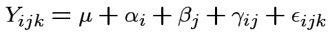
For fixed effects model is
 iid
iid
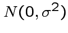 .
.
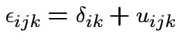
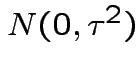
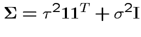
For MANOVA model vector of
is MVN but
with covariance as for ![]() .
.
Intermediate model. Put in subject effect.
Assume
 iid
and
iid
and
 . Then
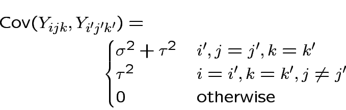
Essentially model says
Do univariate anova: The data reordered:
1 1 1 19
1 1 2 20
1 1 3 18
2 1 1 20
2 1 2 21
2 1 3 19
 et cetera
2 4 2 10
2 4 3 12
3 4 1 11
3 4 2 10
3 4 3 10
4 4 1 11
4 4 2 7
4 4 3 12
The four columns are now labels for subject number, group, scale (a, b or c) and the response. The sas commands:
    data long;
    infile 'table5.7uni';
    input subject group scale score;
run;
proc print;
run;
proc glm;
    class group;
    class scale;
    class subject;
    model score =group subject(group)
                 scale group*scale;
    random subject(group) ;
run;
Some of the output:
Dependent Variable: SCORE
               Sum of    Mean
Source   DF    Squares  Square F    Pr > F
Model    28   843.5333 30.126 19.52 0.0001
Error    34    52.4667  1.543
Total  62   896.0000
Root MSE      SCORE Mean
1.242231        15.33333


Source         DF  TypeISS    MS      F     Pr > F

GROUP           3 743.9000 247.9667 160.69  0.0001
SUBJECT(GROUP) 17  59.4333   3.4961   2.27  0.0208
SCALE           2  21.2381  10.6190   6.88  0.0031
GROUP*SCALE     6  18.9620   3.1603   2.05  0.0860

Source         DF TypeIIISS     MS    F     Pr > F
GROUP           3 743.9000  247.9667 160.69 0.0001
SUBJECT(GROUP) 17  59.4333    3.4961   2.27 0.0208
SCALE           2  16.6242    8.3121   5.39 0.0093
GROUP*SCALE     6  18.9619    3.1603   2.05 0.0860

Source         Type III Expected Mean Square

GROUP          Var(Error) + 3 Var(SUBJECT(GROUP))
                    + Q(GROUP,GROUP*SCALE)
SUBJECT(GROUP) Var(Error) + 3 Var(SUBJECT(GROUP))
SCALE          Var(Error) + Q(SCALE,GROUP*SCALE)
GROUP*SCALE    Var(Error) + Q(GROUP*SCALE)
Type I Sums of Squares:
Type III Sums of Squares:
Notice hypothesis of no group by scale interaction is acceptable.
Under the assumption of no such group by scale interaction the hypothesis of no group effect is tested by dividing group ms by subject(group) ms.
Value is 70.9 on 3,17 degrees of freedom.
This is NOT the F value in the table above since the table above is for FIXED effects.
Notice that the sums of squares in this table match those produced in the repeated measures ANOVA. This is not accidental.