STAT 804: Lecture 20 Notes

Properties of Fourier Series

The Fourier series for a function f truncated to order K, namely

where the coefficients are given by the Fourier integrals gives the best possible approximation to f as a linear combination of these sines and cosines in the following sense. Suppose we try to choose and to minimize

where

Squaring out the integrand and integrating term by term we get, remembering that the sines and cosines are orthogonal,

Taking a derivative with respect to, say, gives which is 0 when is the Fourier coefficient.

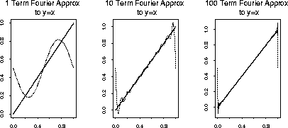
This result says that a Fourier series is the best possible approximation to a function f by a trigonometric polynomial of this type. However, the conclusion depends quite heavily on how we measure the quality of approximation. Below are Fourier approximations to each of 3 functions on [0,1]: the line y=x, the quadratic y=x(1-x) and the square well y=1(x;SPMlt;0.25)+1(y;SPMgt;0.75). For each plot the pictures get better as K improves. However the well shaped plot shows effects of Gibb's phenomenon: near the discontinuity in f there is an overshoot which is very narrow and spiky. The overshoot is of a size which does not depend on the order of approximation.

A simliar discontinuity is implicit in the function y=x since the Fourier approximations are periodic with period 1. This means that the approximations are equal at 0 and at 1 while y=x is not. The quadratic function does have f(0)=f(1) and the Fourier approximation is much better.

My Splus plotting code:

lin <-  function(k)
{
        x <- seq(0, 1, length = 5000)
        kv <- 1:k
        sv <- sin(2 * pi * outer(x, kv))
        y <-  - sv %*% (1/(pi * kv)) + 0.5
        plot(x, x, xlab = "", ylab = "", main = paste(as.character(k), 
                "Term Fourier Approximation to y=x"), type = "l")
        lines(x, y, lty = 2)
}

shows the use of the outer function and the paste function as well as how to avoid loops using matrix arithmetic.