STAT 804: Lecture 21 Notes

The Periodogram

The sample covariance between a series X and is

Using the identity and formulas for geometric sums the mean of the sines can be evaluated. When for an integer k, not 0, we find that so that the sample covariance is simply

For these special we can also compute

so that the sample correlation between X and is just

where is the sample variance .

Consider now adjusting to maximize this correlation. The sine can be rewritten as

so that we are simply choosing coefficients a and b to maximize the correlation between X and subject to the condition . Since correlations are scale invariant we can drop the condition on a and b and miximize the correlation between X and the linear combination of sine and cosine. This problem is solved by linear regression; the coefficients are given by where M is the T by 2 design matrix filled in with the sines and cosines. In fact and we see that the desired regression coefficients are

and

The covariance between X and this best linear combination is

But in fact

which is just the modulus of the discrete Fourier transform divided by T.

Definition: The periodogram is the function

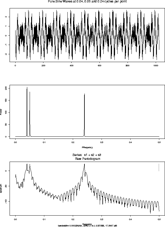
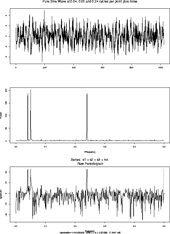
Here are some periodogram plots for some data sets:

• Here is a plot of the modulus of against frequency for the sunspot data. The mean has been subtracted from the data.
  

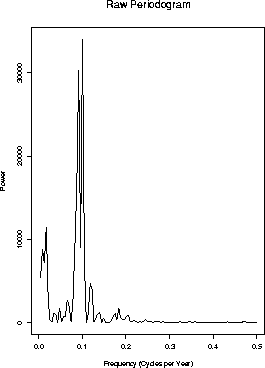
  Notice the peak at a frequency slightly below 0.1 cycles per year as well as a peak at a frequency close to 0.03.

• To get a better understanding of these peaks I plot only for frequencies from 1/12 to 1/8 which should include the largest peak.
  

  Notice that the picture is clearly piecewise linear. This happens because we are actually using the discrete Fourier transform which computes the sample spectrum only at frequencies of the form (in cycles per point) for integer values of K. There are only about 10 points on this plot.

• The same plot against period () shows peaks just below 10 years and just below 11.
  

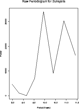
• The DFT can be computed very quickly at the special frequencies but to see the structure clearly near a peak you need to compute for a denser grid of . I use the SPlus function

  transform<- function(x, a, b, n = 100)
  {
          f <- seq(a, b, length = n)
          nn <- 1:length(x)
          args <- outer(f, nn, "*") * 2 * pi
          cosines <- cos(args) * x
          sines <- sin(args) * x
          one <- rep(1, length(x))
          ((cosines %*% one)^2 + (sines %*% one)^2)/length(x)
  }
  

  to compute lots of values for periods between 8 and 12 years.
  

• Now here is the periodogram for the CO2 concentration above Mauna Loa after removing a linear trend from the series by linear regression. Notice the peaks at periods of 1 year and 6 months. These peaks show clearly the annual cycle and the fact that the annual cycle is not a simple sine wave but rather contains overtones: components whose frequency is an integer multiple of the basic frequency of 1 cycle per year.
  

• Now a detail of this image:
  

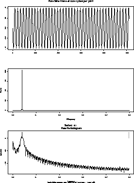
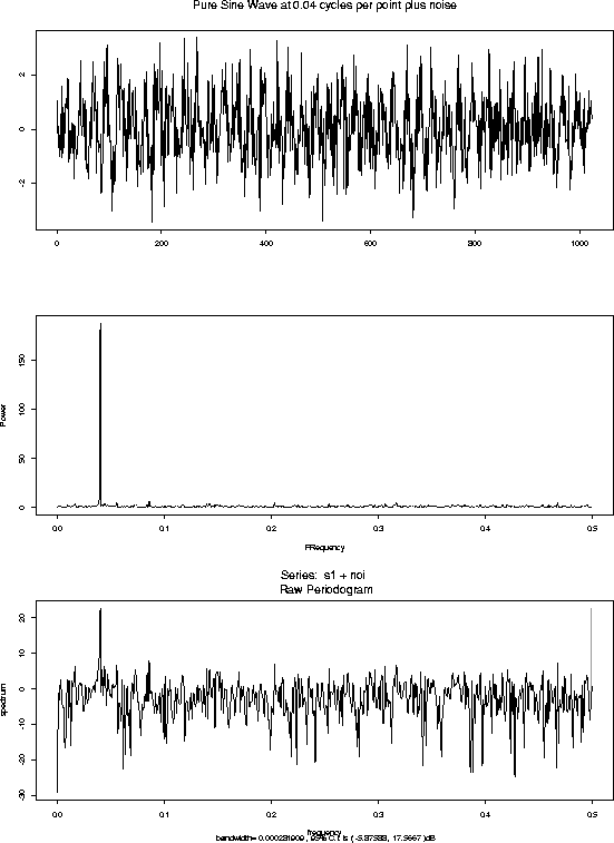
• Here is what the periodogram does with various generated series which have exact sinusoidal components. First a pure sine wave with no noise. The middle panel is a direct plot of the periodogram while the lower panel is the logarithm -- strictly speaking . The apparent waves are actually the effect of round off error in computing the log of something which is algebraically 0 but numerically slightly different.
  

• The same series plus N(01,) white noise. Notice it is much harder to see the perfect sine wave in the data but the periodogram shows the presence of the sine wave quite clearly.
  

• The sum of three sine waves.

• Now add N(0,1) white noise. The periodogram still picks out each of the 3 components very easily.

• The sum of three sine waves.

• Now multiply the pure sine wave by a damping exponential. Notice that the signal is gone by about a quarter of the way through the series. The periodogram still has that peak at 0.04 cycles per point.
  

• Withe noise added you can still see the effect. But compare the scales on the middle plots between all these series.
  

• Now an exponentially damped sine wave plus the other two pure sine waves with N(0,1/16) noise. You can see only two peaks in the raw periodogram but on the logarithmic scale you see that there is a hump on the left of the peak at 0.05 which is the peak at 0.04. The raw scale can make small secondary peaks invisible.
  <\CENTER>