The Problem

For example, consider the function sqrt(x). If x is a perfect square the value can be found exactly, however if x is not a perfect square we know that the result will be irrational. Thus any evaluation of sqrt(x) will be an approximation of the true value.

So if you are given the job of implementing the sqrt function in an application you must figure out some way of approximating the value, quickly and efficiently. Of course most compilers have built in sqrt functions, but somebody had to program these functions in the first place. In addition these arguments hold for a wide range of functions which may or may not be standard compiler functions.

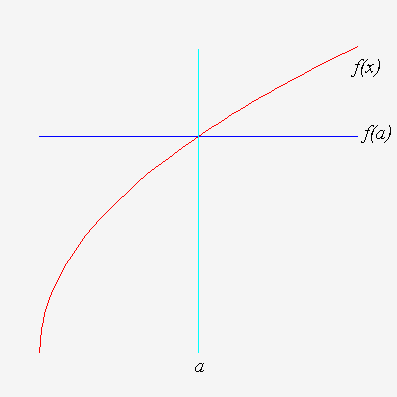
Most approximations of functions happen 'about a point a', the further away from a we go the worse the approximation will be.

Constant Approximations

The simplest approximation is to assume that a function is in fact equal to its value at a nearby point, this is the constant approximation. If we know the value of a function, f, at some point, a, we may assume that it is close to the value of f (a) near a.

Linear Approximations

Of course the constant approximation is not a very good approximation, especially if the slope of the function is steep. A better approximation is to assume that the function is a straight line. The obvious line to take is the tangent line at a, since this will allow for the slope of f near a.

The equation of the tangent line to a function f at a point a is:

y = f '(a) (x - a) + f (a)

f (x) ~ f '(a) (x - a) + f (a)

Example

So our approximation will be

sqrt(x)	~	¼ (x - 4) + 2.
	=	¼ x + 1.

Lets try out our approximation, comparing it with the true value.
> f := x -> sqrt(x);
> ap := x -> x/4 + 1;
> plot([f(x), ap(x)], x = 1..6, color=[red,blue]);
> [evalf(4 + i/10), evalf(f(4 + i/10)), evalf(ap(4 + i/10)), evalf(f(4 + i/10) - ap(4 + i/10))] $ i = -5..5;
From the output we can see that this is not a bad approximation, giving roughly 2 digits accuracy on a range 4 ± 0.5.

1. Write a Maple procedure which takes a function (operator) as input and produces a linear approximation to it at the point approxpoint.
2. Find linear approximations for the following functions about the given points. Graph the function and the approximation on the same graph.
   1. f(x) = x² + 2x + 3, x = 2.
   2. f(x) = ln(x), x = 1.
   3. f(x) = x^1/3, x = 1.
   4. f(x) = 1/(x + 1), x = 1.
   5. f(x) = e^x, x = 0.
   6. f(x) = sin(x), x = 0. Hence conclude that for small x, sin(x) ~ x.
3. Estimate the following using a linear approximation. Compare your approximation with the answer reported by Maple.
   1. ln(2).
   2. The cube root of 2.
   3. e^0.2.
   4. sin(Pi/4).

Error of the Linear Approximation

This shows us that the linear approximation will be good when f ''(x) is small.
If we know a bound for f ''(x) on some interval then we can bound our error.
That is, if | f ''(x) | < M on I, then | E_n(x) | < M | x - a |² on I.

For example, in the case of f (x) = sqrt(x),
D(f )(x) = 1/(2 sqrt(x)),
D(D(f ))(x) = -1/(4 sqrt(x³) < 1/32, if x > 4.
Thus E_n(x) < 1/32 | x - a |² for x > 4.

3. Use the fact that | sin(x) | < 1, and | cos(x) | < 1 to find bounds on the error of the linear approximations to the given functions.
   1. sin(x).
   2. sin(x) + cos(x).

Qudratic Approximations

The reason that the linear approximation works well is that the approximation has the same value at a, and the same slope.
It seems reasonable that we would get an even better approximation if in addition the curvature at a was the same as that of the function. The curvature is measured by the second derivative of f.

Another way of thinking of this is that a linear approximation involves a linear term (x - a), a qudratric approximation will involve the qudratic term (x - a)². Thus we wish to find constants A, B and C such that

Consider P (a) = A. If we want P (a) = f (a) we must have that A = f (a).
Consider P '(x) = B + 2C(x - a), so P '(a) = B, so B = f '(a).
Consider P ''(x) = 2C, so P '(a) = 2C, so C = ½ f ''(a).
Thus the quadratic approximation is given by

The approximation will be better the less the second derivative changes. Thus this is good for functions like sqrt and ln which have relatively slowly changing second derivatives. A function like sin on the other hand has a very variable second derivative and so the approximation will fail more quickly.

Example

Thus f (x) ~ 2 + ¼ (x - 4) - 1/64 (x - 4)²

Using Maple simplify we get that this is 3/4+3/8*x-1/64*x^2.

Lets try some values:
> f := x -> sqrt(x);
> ap := 2 + (x - 4)/4 - (x - 4)^2/64;
> plot([f(x), ap(x)], x = 1..6, color=[red,blue]);
> [evalf(4 + i/10), evalf(f(4 + i/10)), evalf(ap(4 + i/10)), evalf(f(4 + i/10) - ap(4 + i/10))] $ i = -5..5;

We can see that we did indeed get a better approximation, generally 3 digits instead of 2. Near the point the approximation is even better still.

For another example, consider the function ln(x), near 1.
> f := x -> ln(x);
> A := f(1);
> B := D(f)(1);
> C := D(D(f))(1)/2;
> ap := x -> A + B*(x - 1) + C*(x - 1)^2;
> plot([f(x), ap(x)], x = .5..2, color=[red,blue]);
> [evalf(1 + i/10), evalf(f(1 + i/10)), evalf(ap(1 + i/10)), evalf(f(1 + i/10) - ap(1 + i/10))] $ i = -5..5;

1. Write a Maple procedure which takes a function (operator) as input and produces a quadratic approximation to it at the point approxpoint.
2. Find quadratic approximations for the following functions about the given points. Graph the function and the approximation on the same graph.
   1. f(x) = x² + 2x + 3, x = 2.
   2. f(x) = ln(x), x = 1.
   3. f(x) = x^1/3, x = 1.
   4. f(x) = 1/(x + 1), x = 1.
   5. f(x) = e^x, x = 0.
   6. f(x) = sin(x), x = Pi/2.
3. Estimate the following using a quadratic approximation. Compare your approximation with the answer reported by Maple and with the answer you got for a linear approximation.
   1. ln(2).
   2. The cube root of 2.
   3. e^0.2.
   4. sin(Pi/4).

Error of the Quadratic Approximation

This shows us that the linear approximation will be good when f '''(x) is small, i.e. the second derivative is changing slowly.
If we know a bound for f '''(x) on some interval then we can bound our error.
That is, if | f '''(x) | < M on I, then | E_n(x) | < M | x - a |³ on I.

In the case of f(x) = sqrt(x),
D(f )(x) = 1/(2 sqrt(x)),
D(D(f ))(x) = -1/(4 sqrt(x³)
(D@@3)(f)(x) = 3/(8 sqrt(x⁵)
So (D@@3)(f)(5) = 1/256.
Thus E_n(x) < 1/256 (x - a)³, for x > 4.

3. Use the fact that |sin(x)| < 1, and |cos(x)| < 1 to find bounds on the error of the quadratric approximations to the given functions.
   1. sin(x).
   2. sin(x) + cos(x).

Up to Main Lab Page

Next Lesson - Taylor Series

Previous Lesson - Text in Maple

Top of this Lesson