The idea of numerical integration is to find the value of the integral of f (x) from a to b by estimating the area under the curve from a to b, counting areas below the axis as negative.

The Midpoint Rule

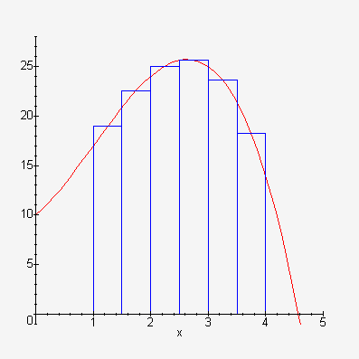
In this definition the integral is taken to be the limit of a sum of areas. If we instead take a finite number, n, of subintervals we will get an approximation to the integral. We choose x_i^* to be the midpoint of each subinterval. i.e. x_i^* = ½( x_i-1 + x_i ), for each i from 1 to n.

The area of each rectangle is f ( x_i^* ) x.
Since each rectangle has the same width: x = (b - a)/n
x_i^* = ½( x_i-1 + x_i ).

So f (x) dx ~ (b - a)/n ( f ( x₁^* ) + f ( x₂^* ) + . . . + f ( x_n^* ) ), where x_i^* = ½( x_i-1 + x_i ).

Example

Now we can use the procedure to find the value for various values of n, and compare them to the value reported by Maple.
> f:= x -> exp(x)*sin(x);
> evalf(int(f(x), x = 0..Pi));
> midp(f, 0, Pi, 10);
> midp(f, 0, Pi, 20);
> midp(f, 0, Pi, 50);
> midp(f, 0, Pi, 100);

1. Use the midpoint method to estimate the following integrals, using n = 5, 10 and 50. Where possible check your answers with the Maple int function.
   1. exp(1/x), from 1 to 2.
   2. -exp(-x)/x, from 1 to 2.
   3. (1/sqrt(2*Pi)) * exp(-(t^2)/2) from -2 to 2.
   4. sin(x^2)*exp(x), from 1 to 2.

Error Analysis

The Trapezoidal Rule

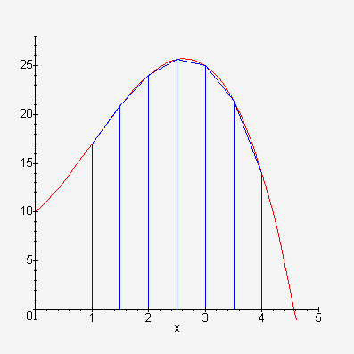
A better approach is to estimate the area under each subinterval by a trapezoid (a rectangle with a triangle on top). We take the top of the trapezoid to be the secant line from f (x_i-1) to f (x_i).

The area of each trapezoid is the area of the rectangle with width x and height f (x_i-1) plus the area of the triangle with base x and height f (x_i) - f (x_i-1).

Thus the area of the trapezoid is x f (x_i-1) + ½ x ( f (x_i) - f (x_i-1)) = ½ x ( f (x_i-1) + f (x_i))

Now consider the sum of these terms;
½ x ( f (x₀) + f (x₁) ) + ½ x ( f (x₁) + f (x₂) ) + ½ x ( f (x₂) + f (x₃) ) + . . . + ½ x ( f (x_n-1) + f (x_n) )
= ½ x ( (f (x₀) + f (x₁) ) + (f (x₁) + f (x₂) ) + (f (x₂) + f (x₃) ) + . . . f (x_n-1) + f (x_n) )

Since each term except the first and last appears twice we can simplify this to get the fromula for the Trapezoidal rule:

f (x) dx ~ (b - a)/n ( f (x₀) + 2f (x₁) + 2f (x₂) + . . . + 2 f (x_n-1) + f (x_n)).

Example

> trap := proc(f, a::realcons, b::realcons, n::integer)
> local dx, i, sm;
> dx := (b - a)/n;
> sm := 0;
> for i from evalf(a+dx) by evalf(dx) to evalf(b-dx) do
> sm := evalf(sm + 2*f(i));
> od;
> RETURN(evalf(dx*(sm + f(a) + f(b))/2));
> end;

Now we can use the procedure to find the value for various values of n, and compare them to the value reported by Maple.
> f:= x -> exp(x)*sin(x);
> evalf(int(f(x), x = 0..Pi));
> trap(f, 0, Pi, 10);
> trap(f, 0, Pi, 20);
> trap(f, 0, Pi, 50);
> trap(f, 0, Pi, 100);

2. Use the Trapezoidal rule to estimate the following integrals, using n = 5, 10 and 50. Where possible check your answers with the Maple int function.
   1. exp(1/x), from 1 to 2.
   2. -exp(-x)/x, from 1 to 2.
   3. (1/sqrt(2*Pi)) * exp(-(t^2)/2) from -2 to 2.
   4. sin(x^2)*exp(x), from 1 to 2));

Error Analysis

Simpson's Rule

We will adopt the notation that h = x, and y_i = f (x_i).

So with is notation we will use the area under parabola which goes through the points (x₀, y₀) (x₁, y₁) (x₂, y₂) for our first area.
The area under parabola which goes through the points (x₂, y₂) (x₃, y₃) (x₄, y₄) for our second area and so on.

Suppose first that our points are (-h, y₀) (0, y₁), (h, y₂), and that our parabola has the form A x² + B x + C. Then the area under it from -h to h is given by:
> P := x -> A*x^2 + B*x + C;
> int(P(x), x = -h..h);

Now, we know that this porabola goes through the points (-h, y₀) (0, y₁), (h, y₂).
Thus y₀ = P (-h)
y₁ = P (0)
y₂ = P (h)
Substituting these values in our polynomial gives
> P(-h);
> P(0);
> P(h);
> P(-h) + 4*P(0) + P(h);
Simpson noticed that h/3 (y₀ + 4 y₁ + y₂) = 2/3 Ah³ + 2Ch = the area under the parabola.

Since moving the parabola left or right does not change the area under it we can use this formula for any three points, whether or not they are centered at 0. Thus in general the area under the parabola through the points (x_i-1, y_i-1) (x_i, y_i) (x_i+1, y_i+1) from x_i-1 to x_i+1 is given by h/3 (y_i-1 + 4 y_i + y_i+1).

So the integral of f (x) from a to b can be approximated by:
h/3 (y₀ + 4 y₁ + y₂) + h/3 (y₂ + 4 y₃ + y₄) + . . . + h/3 (y_n-2 + 4 y_n-1 + y_n)
Simplifying gives us Simpson's Rule:

f (x) dx ~ (b - a)/(3n) ( y₀ + 4 y₁ + 2 y₂ + 4 y₃ + 2 y₄ + . . . + 2 y_n-2 + 4 y_n-1 + y_n).

Notice the pattern of the coefficients 1, 2, 4, 2, 4, . . . , 4, 2, 4, 1.

Example

> simpson := proc(f, a::realcons, b::realcons, n::even)
> local h, i, sm, x;
> h := (b - a)/n;
> sm := 0;
> for i from 1 to n-1 do
> x := a + i * h;
> if type(i, even) then
> sm := sm + 2*f(x);
> else
> sm := sm + 4*f(x);
> fi;
> od;
> RETURN(evalf(h/3*(sm + f(a) + f(b))));
> end;

Now we can use the procedure to find the value for various values of n, and compare them to the value reported by Maple.
> f:= x -> exp(x)*sin(x);
> evalf(int(f(x), x = 0..Pi));
> simpson(f, 0, Pi, 10);
> simpson(f, 0, Pi, 20);
> simpson(f, 0, Pi, 50);
> simpson(f, 0, Pi, 100);

It is clear that Simpson Rule is a vast improvement over either the midpoint or the Trapezoidal rules.

1. Use Simpson's rule to estimate the following integrals, using n = 5, 10 and 50. Where possible check your answers with the Maple int function. Also compare your results with those obtained by using the Midpoint and Trapezoidal rules.
   1. exp(1/x), from 1 to 2.
   2. -exp(-x)/x, from 1 to 2.
   3. (1/sqrt(2*Pi)) * exp(-(t^2)/2) from -2 to 2.
   4. sin(x^2)*exp(x), from 1 to 2));

Error Analysis

Up to Main Lab Page

Next Lesson - Differential Equations

Previous Lesson - Integration

Top of this Lesson