Example 11.2: Interpolating Irregular Observations

The EXPAND Procedure

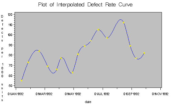
Example 11.2: Interpolating Irregular Observations

This example shows the interpolation of a series of values measured at irregular points in time. The data are hypothetical. Assume that a series of randomly timed quality control inspections are made and defect rates for a process are measured. The problem is to produce two reports: estimates of monthly average defect rates for the months within the period covered by the samples, and a plot of the interpolated defect rate curve over time.

The following statements read and print the input data, as shown in Output 11.2.1.

   data samples;
     input date : date9. defects @@;
     label defects = "Defects per 1000 units";
     format date date9.;
   datalines;
   13jan1992    55    27jan1992   73    19feb1992   84    8mar1992   69
   27mar1992    66     5apr1992   77    29apr1992   63   11may1992   81
   25may1992    89     7jun1992   94    23jun1992  105   11jul1992   97
   15aug1992   112    29aug1992   89    10sep1992   77   27sep1992   82
   ;
   
   title "Sampled Defect Rates";
   proc print data=samples;
   run;

Output 11.2.1: Measured Defect Rates

Sampled Defect Rates

Obs	date	defects
1	13JAN1992	55
2	27JAN1992	73
3	19FEB1992	84
4	08MAR1992	69
5	27MAR1992	66
6	05APR1992	77
7	29APR1992	63
8	11MAY1992	81
9	25MAY1992	89
10	07JUN1992	94
11	23JUN1992	105
12	11JUL1992	97
13	15AUG1992	112
14	29AUG1992	89
15	10SEP1992	77
16	27SEP1992	82

To compute the monthly estimates, use PROC EXPAND with the TO=MONTH option and specify OBSERVED=(BEGINNING,AVERAGE). The following statements interpolate the monthly estimates.

   proc expand data=samples out=monthly to=month;
     id date;
     convert defects / observed=(beginning,average);
   run;
   
   title "Estimated Monthly Average Defect Rates";
   proc print data=monthly;
   run;

The results are printed in Output 11.2.2.

Output 11.2.2: Monthly Average Estimates

Estimated Monthly Average Defect Rates

Obs	date	defects
1	JAN1992	59.323
2	FEB1992	82.000
3	MAR1992	66.909
4	APR1992	70.205
5	MAY1992	82.762
6	JUN1992	99.701
7	JUL1992	101.564
8	AUG1992	105.491
9	SEP1992	79.206

To produce the plot, first use PROC EXPAND with TO=DAY to interpolate a full set of daily values, naming the interpolated series INTERPOL. Then merge this data set with the samples so you can plot both the measured and the interpolated values on the same graph. PROC GPLOT is used to plot the curve. The actual sample points are plotted with asterisks. The following statements interpolate and plot the defects rate curve.

   proc expand data=samples out=daily to=day;
     id date;
     convert defects = interpol;
   run;
   
   data daily;
     merge daily samples;
     by date;
   run;
   
   title "Plot of Interpolated Defect Rate Curve";
   proc gplot data=daily; 
      axis2 label=(a=-90 r=90 );
      symbol1 v=none i=join;
      symbol2 v=star i=none;
      plot interpol * date = 1 defects * date = 2  / 
           vaxis=axis2 overlay;
   run;
   quit;

The plot is shown in Output 11.2.3.

Output 11.2.3: Interpolated Defects Rate Curve

Chapter Contents
Previous
Next
Top