Solution Modes

Chapter Contents

The MODEL Procedure

Solution Modes

The following solution modes are commonly used:

Dynamic simultaneous forecast mode is used for forecasting with the model. Collect the historical data on the model variables, the future assumptions of the exogenous variables, and any prior information on the future endogenous values, and combine them in a SAS data set. Use the FORECAST option on the SOLVE statement.
Dynamic simultaneous simulation mode is often called ex-post simulation, historical simulation, or ex-post forecasting. Use the DYNAMIC option. This mode is the default.
Static simultaneous simulation mode can be used to examine the within-period performance of the model without the complications of previous period errors. Use the STATIC option.
NAHEAD=n dynamic simultaneous simulation mode can be used to see how well n-period-ahead forecasting would have performed over the historical period. Use the NAHEAD=n option.

The different solution modes are explained in detail in the following sections.

Dynamic and Static Simulations

In model simulation, either solved values or actual values from the data set can be used to supply lagged values of an endogenous variable. A dynamic solution refers to a solution obtained by using only solved values for the lagged values. Dynamic mode is used both for forecasting and for simulating the dynamic properties of the model.

A static solution refers to a solution obtained by using the actual values when available for the lagged endogenous values. Static mode is used to simulate the behavior of the model without the complication of previous period errors. Dynamic simulation is the default.

If you wish to use static values for lags only for the first n observations, and dynamic values thereafter, specify the START=n option. For example, if you want a dynamic simulation to start after observation twenty-four, specify START=24 on the SOLVE statement. If the model being simulated had a value lagged for four time periods, then this value would start using dynamic values when the simulation reached observation number 28.

n-Period-Ahead Forecasting

Suppose you want to regularly forecast 12 months ahead and produce a new forecast each month as more data becomes available. n-period-ahead forecasting allows you to test how well you would have done over time had you been using your model to forecast 1 year ahead.

To see how well a model predicts n time periods in the future, perform an n-period-ahead forecast on real data and compare the forecast values with the actual values.

n-period-ahead forecasting refers to using dynamic values for the lagged endogenous variables only for lags 1 through n-1. For example, 1-period-ahead forecasting, specified by the NAHEAD=1 option on the SOLVE statement, is the same as if a static solution had been requested. Specifying NAHEAD=2 produces a solution that uses dynamic values for lag one and static, actual, values for longer lags.

The following example is a 2-year-ahead dynamic simulation. The output is shown in Figure 14.59.

   data yearly;
      input year x1 x2 x3 y1 y2 y3;
      datalines;
   84 4 9  0  7  4  5
   85 5 6  1  1  27  4
   86 3 8  2  5  8  2
   87 2 10 3  0  10 10
   88 4 7  6  20 60 40
   89 5 4  8  40 40 40
   90 3 2  10 50 60 60
   91 2 5  11 40 50 60
   ;
   run;
   
   proc model data=yearly outmodel=foo;
      endogenous y1 y2 y3;
      exogenous  x1 x2 x3;
   
      y1 = 2 + 3*x1 - 2*x2 + 4*x3;
      y2 = 4 + lag2( y3 ) + 2*y1 + x1;
      y3 = lag3( y1 ) + y2 - x2;
   
      solve y1 y2 y3 / nahead=2 out=c;
   run;
   
   proc print data=c;run;

The MODEL Procedure

Dynamic Simultaneous 2-Periods-Ahead Forecasting Simulation

Data Set Options
DATA=	YEARLY
OUT=	C

Solution Summary
Variables Solved	3
Simulation Lag Length	3
Solution Method	NEWTON
CONVERGE=	1E-8
Maximum CC	0
Maximum Iterations	1
Total Iterations	8
Average Iterations	1

Observations Processed
Read	20
Lagged	12
Solved	8
First	5
Last	8

Variables Solved For	y1 y2 y3

Figure 14.59: NAHEAD Summary Report

Obs	_TYPE_	_MODE_	_LAG_	_ERRORS_	y1	y2	y3	x1	x2	x3
1	PREDICT	SIMULATE	0	0	0	10	7	2	10	3
2	PREDICT	SIMULATE	1	0	24	58	52	4	7	6
3	PREDICT	SIMULATE	1	0	41	101	102	5	4	8
4	PREDICT	SIMULATE	1	0	47	141	139	3	2	10
5	PREDICT	SIMULATE	1	0	42	130	145	2	5	11

Figure 14.60: C Data Set

The proceding 2-year-ahead simulation can be emulated without using the NAHEAD= option by the following PROC MODEL statements:

   proc model data=test model=foo;
     range year = 87 to 88;
     solve y1 y2 y3 / dynamic solveprint;
   run;
   
     range year = 88 to 89;
     solve y1 y2 y3 / dynamic solveprint;
   run;
   
     range year = 89 to 90;
     solve y1 y2 y3 / dynamic solveprint;
   run;
   
     range year = 90 to 91;
     solve y1 y2 y3 / dynamic solveprint;

The totals shown under "Observations Processed" in Figure 14.59 are equal to the sum of the four individual runs.

Simulation and Forecasting

You can perform a simulation of your model or use the model to produce forecasts. Simulation refers to the determination of the endogenous or dependent variables as a function of the input values of the other variables, even when actual data for some of the solution variables are available in the input data set. The simulation mode is useful for verifying the fit of the model parameters. Simulation is selected by the SIMULATE option on the SOLVE statement. Simulation mode is the default.

In forecast mode, PROC MODEL solves only for those endogenous variables that are missing in the data set. The actual value of an endogenous variable is used as the solution value whenever nonmissing data for it are available in the input data set. Forecasting is selected by the FORECAST option on the SOLVE statement. For example, an econometric forecasting model can contain an equation to predict future tax rates, but tax rates are usually set in advance by law. Thus, for the first year or so of the forecast, the predicted tax rate should really be exogenous. Or, you may want to use a prior forecast of a certain variable from a short-run forecasting model to provide the predicted values for the earlier periods of a longer-range forecast of a long-run model. A common situation in forecasting is when historical data needed to fill the initial lags of a dynamic model are available for some of the variables but have not yet been obtained for others. In this case, the forecast must start in the past to supply the missing initial lags. Clearly, you should use the actual data that are available for the lags. In all the preceding cases, the forecast should be produced by running the model in the FORECAST mode; simulating the model over the future periods would not be appropriate.

Monte Carlo Simulation

The accuracy of the forecasts produced by PROC MODEL depends on four sources of error (Pindyck 1981, 405-406):

The system of equations contains an implicit random error term ${\epsilon}$
$g(y,x,\hat{{{\theta}}})={{\epsilon}}$
where y, x, g, ${\hat{{{\theta}}}}$ , and ${\epsilon}$ are vector valued.
The estimated values of the parameters, ${\hat{{{\theta}}}}$ , are themselves random variables.
The exogenous variables may have been forecast themselves and therefore may contain errors.
The system of equations may be incorrectly specified; the model only approximates the process modeled.

The RANDOM= option is used to request Monte Carlo (or stochastic) simulations to generate confidence intervals for errors arising from the first two sources. The Monte Carlo simulations can be performed with ${\epsilon}$ , ${\theta}$ , or both vectors represented as random variables. The SEED= option is used to control the random number generator for the simulations. SEED=0 forces the random number generator to use the system clock as its seed value.

In Monte Carlo simulations, repeated simulations are performed on the model for random perturbations of the parameters and the additive error term. The random perturbations follow a multivariate normal distribution with expected value of 0 and covariance described by a covariance matrix of the parameter estimates in the case of ${\theta}$ ,or a covariance matrix of the equation residuals for the case of ${\epsilon}$ . PROC MODEL can generate both covariance matrices or you can provide them.

The ESTDATA= option specifies a data set containing an estimate of the covariance matrix of the parameter estimates to use for computing perturbations of the parameters. The ESTDATA= data set is usually created by the FIT statement with the OUTEST= and OUTCOV options. When the ESTDATA= option is specified, the matrix read from the ESTDATA= data set is used to compute vectors of random shocks or perturbations for the parameters. These random perturbations are computed at the start of each repetition of the solution and added to the parameter values. The perturbed parameters are fixed throughout the solution range. If the covariance matrix of the parameter estimates is not provided, the parameters are not perturbed.

The SDATA= option specifies a data set containing the covariance matrix of the residuals to use for computing perturbations of the equations. The SDATA= data set is usually created by the FIT statement with the OUTS= option. When SDATA= is specified, the matrix read from the SDATA= data set is used to compute vectors of random shocks or perturbations for the equations. These random perturbations are computed at each observation. The simultaneous solution satisfies the model equations plus the random shocks. That is, the solution is not a perturbation of a simultaneous solution of the structural equations; rather, it is a simultaneous solution of the stochastic equations using the simulated errors. If the SDATA= option is not specified, the random shocks are not used.

The different random solutions are identified by the _REP_ variable in the OUT= data set. An unperturbed solution with _REP_=0 is also computed when the RANDOM= option is used. RANDOM=n produces n+1 solution observations for each input observation in the solution range. If the RANDOM= option is not specified, the SDATA= and ESTDATA= options are ignored, and no Monte Carlo simulation is performed.

PROC MODEL does not have an automatic way of modeling the exogenous variables as random variables for Monte Carlo simulation. If the exogenous variables have been forecast, the error bounds for these variables should be included in the error bounds generated for the endogenous variables. If the models for the exogenous variables are included in PROC MODEL, then the error bounds created from a Monte Carlo simulation will contain the uncertainty due to the exogenous variables.

Alternatively, if the distribution of the exogenous variables is known, the built-in random number generator functions can be used to perturb these variables appropriately for the Monte Carlo simulation. For example, if you knew the forecast of an exogenous variable, X, had a standard error of 5.2 and the error was normally distributed, then the following statements could be used to generate random values for X:

   x_new = x + 5.2 * rannor(456);

During a Monte Carlo simulation the random number generator functions produce one value at each observation. It is important to use a different seed value for all the random number generator functions in the model program; otherwise, the perturbations will be correlated. For the unperturbed solution, _REP_=0, the random number generator functions return 0.

PROC UNIVARIATE can be used to create confidence intervals for the simulation (see the Monte Carlo simulation example in the "Getting Started" section).

Quasi-Random Number Generators

Traditionally high discrepancy psuedo-random number generators are used to generate innovations in Monte Carlo simulations. Loosely translated, a high discrepancy psuedo-random number generator is one in which there is very little correlation between the current number generated and the past numbers generated. This property is ideal if indeed independance of the innovations is required. If, on the other hand, the efficient spanning of a multi-dimensional space is desired, a low discrepancy, quasi-random number generator can be used. A quasi-random number generator produces numbers which have no random component.

A simple one-dimensional quasi-random sequence is the van der Corput sequence. Given a prime number r ( r>=2 ) any integer has a unique representation in terms of base r. A number in the interval [0,1) can be created by inverting the represention base power by base power. For example, consider r=3 and n=1. 1 in base 3 is

1₁₀ = 1 ·3⁰ = 1₃

When the powers of 3 are inverted,

$\phi(1) = \frac{1}3$

Also 11 in base 3 is

11₁₀ = 1 ·3² + 2 ·3⁰ = 102₃

When the powers of 3 are inverted,

$\phi(11) = \frac{1}9 + 2\cdot\frac{1}3 = \frac{7}9$

The first 10 numbers in this squence $\phi(1) ... \phi(10)$ are provided below

0, (1/3), (2/3), (1/9), (4/9), (7/9), (2/9), (5/9), (8/9), (1/27)

As the sequence proceeds it fills in the gaps in a uniform fashion.

Several authors have expanded this idea to many dimensions. Two versions supported by the MODEL procedure are the Sobol sequence (QUASI=SOBOL) and the Faure sequence (QUASI=FAURE). The Sobol sequence is based on binary numbers an is generally computationaly faster than the Faure sequence. The Faure sequence uses the dimensionality of the problem to determine the number base to use to generate the sequence. The Faure sequence has better distributional properties than the Sobol sequence for dimensions greater than 8.

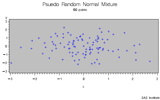
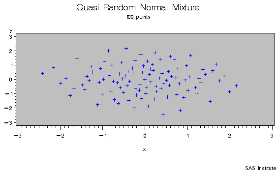
As an example of the difference between a pseudo random number and a quasi random number consider simulating a bivariate normal with 100 draws.

Figure 14.61: A Bivariate Normal using 100 pseudo random draws

Figure 14.62: A Bivariate Normal using 100 Faure random draws

Solution Mode Output

The following SAS statements dynamically forecast the solution to a nonlinear equation:

   proc model data=sashelp.citimon;
      parameters a 0.010708  b  -0.478849 c 0.929304;
      lhur = 1/(a * ip) + b + c * lag(lhur);
      solve lhur / out=sim forecast dynamic;
   run;

The first page of output produced by the SOLVE step is shown in Figure 14.63. This is the summary description of the model. The error message states that the simulation was aborted at observation 144 because of missing input values.

The MODEL Procedure

Model Summary
Model Variables	1
Parameters	3
Equations	1
Number of Statements	1
Program Lag Length	1

Model Variables	LHUR
Parameters	a(0.010708) b(-0.478849) c(0.929304)
Equations	LHUR

The MODEL Procedure

Dynamic Single-Equation Forecast

ERROR: Solution values are missing because of missing input values for observation 144 at NEWTON iteration 0.

NOTE: Additional information on the values of the variables at this observation, which may be helpful in determining the cause of the failure of the solution process, is printed below.

Iteration Errors - Missing.

NOTE: Simulation aborted.

Figure 14.63: Solve Step Summary Output

The second page of output, shown in Figure 14.64, gives more information on the failed observation.

The MODEL Procedure

Dynamic Single-Equation Forecast

ERROR: Solution values are missing because of missing input values for observation 144 at NEWTON iteration 0.

NOTE: Additional information on the values of the variables at this observation, which may be helpful in determining the cause of the failure of the solution process, is printed below.

Observation	144	Iteration	0	CC	-1.000000
		Missing	1

Iteration Errors - Missing.

_N_: 144 ACTUAL.LHUR: . ERROR.LHUR: . IP: . LHUR: 7.10000 PRED.LHUR: . RESID.LHUR: . a: 0.01071 b: -0.47885 c: 0.92930

NOTE: Simulation aborted.

Figure 14.64: Solve Step Error Message

From the program data vector you can see the variable IP is missing for observation 144. LHUR could not be computed so the simulation aborted.

The solution summary table is shown in Figure 14.65.

The MODEL Procedure

Dynamic Single-Equation Forecast

Data Set Options
DATA=	SASHELP.CITIMON
OUT=	SIM

Solution Summary
Variables Solved	1
Forecast Lag Length	1
Solution Method	NEWTON
CONVERGE=	1E-8
Maximum CC	0
Maximum Iterations	1
Total Iterations	143
Average Iterations	1

Observations Processed
Read	145
Lagged	1
Solved	143
First	2
Last	145
Failed	1

Variables Solved For	LHUR

Figure 14.65: Solution Summary Report

This solution summary table includes the names of the input data set and the output data set followed by a description of the model. The table also indicates the solution method defaulted to Newton's method. The remaining output is defined as follows:

Maximum CC is the maximum convergence value accepted by the Newton

procedure. This number is always less than the value

for "CONVERGE=."

Maximum Iterations is the maximum number of Newton iterations performed

at each observation and each replication of Monte

Carlo simulations.

Total Iterations is the sum of the number of iterations required for each

observation and each Monte Carlo simulation.

Average Iterations is the average number of Newton iterations required to

solve the system at each step.

Solved is the number of observations used times the number of

random replications selected plus one, for Monte Carlo

simulations. The one additional simulation is the original

unperturbed solution. For simulations not involving Monte

Carlo, this number is the number of observations used.

Summary Statistics

The STATS and THEIL options are used to select goodness of fit statistics. Actual values must be provided in the input data set for these statistics to be printed. When the RANDOM= option is specified, the statistics do not include the unperturbed (_REP_=0) solution.

STATS Option Output

If the STATS and THEIL options are added to the model in the previous section

   proc model data=sashelp.citimon;
      parameters a 0.010708  b  -0.478849 c 0.929304;
      lhur= 1/(a * ip) + b + c * lag(lhur) ;
      solve lhur / out=sim dynamic stats theil;
      range date to '01nov91'd;
   run;

the STATS output in Figure 14.66 and the THEIL output in Figure 14.67 are generated.

The MODEL Procedure

Dynamic Single-Equation Simulation

Solution Range DATE = FEB1980 To NOV1991

Descriptive Statistics
Variable	N Obs	N	Actual		Predicted		Label
Variable	N Obs	N	Mean	Std Dev	Mean	Std Dev	Label
LHUR	142	142	7.0887	1.4509	7.2473	1.1465	UNEMPLOYMENT RATE: ALL WORKERS, 16 YEARS

Statistics of fit
Variable	N	Mean Error	Mean % Error	Mean Abs Error	Mean Abs % Error	RMS Error	RMS % Error	R-Square	Label
LHUR	142	0.1585	3.5289	0.6937	10.0001	0.7854	11.2452	0.7049	UNEMPLOYMENT RATE: ALL WORKERS, 16 YEARS

Figure 14.66: STATS Output

The number of observations (Nobs), the number of observations with both predicted and actual values nonmissing (N), and the mean and standard deviation of the actual and predicted values of the determined variables are printed first. The next set of columns in the output are defined as follows:

Mean Error ${{1 \over N}\sum_{j=1}^N{(\hat{y}_{j} - y_{j} )}}$

Mean % Error ${{100 \over N}\sum_{j=1}^N{(\hat{y}_{j} - y_{j}) / y_{j}}}$

Mean Abs Error ${{1 \over N}\sum_{j=1}^N{|{\hat{y}_{j} - y_{j} }|}}$

Mean Abs % Error ${{100 \over N}\sum_{j=1}^N{{|(\hat{y}_{j} - y_{j})/ y_{j}|}}}$

RMS Error ${\sqrt{{1 \over N}\sum_{j=1}^N{(\hat{y}_{j} - y_{j})^2}}}$

RMS % Error ${100\sqrt{{1 \over N}\sum_{j=1}^N{((\hat{y}_{j} - y_{j})/ y_{j})^2}}}$

R-square 1 - SSE / CSSA

SSE ${\sum_{j=1}^N{(\hat{y}_{j} - y_{j} )^2}}$

SSA ${\sum_{j=1}^N{(y_{j} )^2}}$

CSSA ${{SSA} - (\sum_{j=1}^N{y_{j} } )^2}$

${\hat y}$ predicted value

y actual value

When the RANDOM= option is specified, the statistics do not include the unperturbed (_REP_=0) solution.

THEIL Option Output

The THEIL option specifies that Theil forecast error statistics be computed for the actual and predicted values and for the relative changes from lagged values. Mathematically, the quantities are

$\hat{yc} = (\hat{y} - lag(y)) / lag(y)$

yc = (y - lag(y)) / lag(y)

where ${\hat yc}$ is the relative change for the predicted value and yc is the relative change for the actual value.

The MODEL Procedure

Dynamic Single-Equation Simulation

Solution Range DATE = FEB1980 To NOV1991

Theil Forecast Error Statistics
Variable	N	MSE	Corr (R)	MSE Decomposition Proportions					Inequality Coef		Label
Variable	N	MSE	Corr (R)	Bias (UM)	Reg (UR)	Dist (UD)	Var (US)	Covar (UC)	U1	U	Label
LHUR	142.0	0.6168	0.85	0.04	0.01	0.95	0.15	0.81	0.1086	0.0539	UNEMPLOYMENT RATE: ALL WORKERS, 16 YEARS

Theil Relative Change Forecast Error Statistics
Variable	Relative Change			MSE Decomposition Proportions					Inequality Coef		Label
Variable	N	MSE	Corr (R)	Bias (UM)	Reg (UR)	Dist (UD)	Var (US)	Covar (UC)	U1	U	Label
LHUR	142.0	0.0126	-0.08	0.09	0.85	0.06	0.43	0.47	4.1226	0.8348	UNEMPLOYMENT RATE: ALL WORKERS, 16 YEARS

Figure 14.67: THEIL Output

The columns have the following meaning:

Corr (R)

is the correlation coefficient, ${{\rho}}$ , between the actual and predicted values.

${\rho} = \frac{\rm{cov}( y, \hat{y})} { {\sigma}_{a} {\sigma}_{p}}$

where ${{\sigma}_{p}}$ and ${{\sigma}_{a}}$ are the standard deviations of the predicted and actual values.

Bias (UM)

is an indication of systematic error and measures the extent to which the average values of the actual and predicted deviate from each other.

$\frac{(\rm{E}(y)- \rm{E}(\hat{y}))^2} { \frac{1}N \sum_{t=1}^N{(y_{t} - \hat{y}_{t})^2} }$

Reg (UR)

is defined as ${({\sigma}_{p} - {\rho} * {\sigma}_{a})^2/ {MSE}}$ .Consider the regression

$y = {\alpha}+ {\beta}\hat{y}$

If ${\hat{{\beta}}=1}$ , UR will equal zero.

Dist (UD)

is defined as ${(1 - {\rho}^2) {\sigma}_{a}{\sigma}_{a}/{MSE}}$ and represents the variance of the residuals obtained by regressing yc on ${\hat yc}$ .

Var (US)

is the variance proportion. US indicates the ability of the model to replicate the degree of variability in the endogenous variable.

${US} = \frac{({\sigma}_{p}-{\sigma}_{a})^2}{MSE}$

Covar (UC)

represents the remaining error after deviations from average values and average variabilities have been accounted for.

${UC} = \frac{2(1 - {\rho}) {\sigma}_{p}{\sigma}_{a}}{MSE}$

U1

is a statistic measuring the accuracy of a forecast.

${U1}=\frac{MSE}{\sqrt{{1 \over N}\sum_{t=1}^N{(y_{t})^2}}}$

U

is the Theil's inequality coefficient defined as follows:

$U=\frac{MSE} {\sqrt{{1 \over N}\sum_{t=1}^N{(y_{t})^2}} + \sqrt{{1 \over N}\sum_{t=1}^N{( \hat{y}_{t})^2}}}$

MSE

is the mean square error

${MSE} = \frac{1}N \sum_{t=1}^N{(\hat{yc} - yc)^2}$

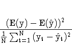
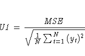
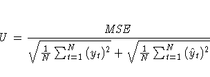
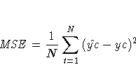
More information on these statistics can be found in the references Maddala (1977, 344--347) and Pindyck and Rubinfeld (1981, 364 -365).

Chapter Contents
Previous
Next
Top

Maximum CC	is the maximum convergence value accepted by the Newton
	procedure. This number is always less than the value
	for "CONVERGE=."
Maximum Iterations	is the maximum number of Newton iterations performed
	at each observation and each replication of Monte
	Carlo simulations.
Total Iterations	is the sum of the number of iterations required for each
	observation and each Monte Carlo simulation.
Average Iterations	is the average number of Newton iterations required to
	solve the system at each step.
Solved	is the number of observations used times the number of
	random replications selected plus one, for Monte Carlo
	simulations. The one additional simulation is the original
	unperturbed solution. For simulations not involving Monte
	Carlo, this number is the number of observations used.

Mean Error	${{1 \over N}\sum_{j=1}^N{(\hat{y}_{j} - y_{j} )}}$

Mean % Error	${{100 \over N}\sum_{j=1}^N{(\hat{y}_{j} - y_{j}) / y_{j}}}$

Mean Abs Error	${{1 \over N}\sum_{j=1}^N{\|{\hat{y}_{j} - y_{j} }\|}}$

Mean Abs % Error	${{100 \over N}\sum_{j=1}^N{{\|(\hat{y}_{j} - y_{j})/ y_{j}\|}}}$

RMS Error	${\sqrt{{1 \over N}\sum_{j=1}^N{(\hat{y}_{j} - y_{j})^2}}}$

RMS % Error	${100\sqrt{{1 \over N}\sum_{j=1}^N{((\hat{y}_{j} - y_{j})/ y_{j})^2}}}$

R-square	1 - SSE / CSSA

SSE	${\sum_{j=1}^N{(\hat{y}_{j} - y_{j} )^2}}$

SSA	${\sum_{j=1}^N{(y_{j} )^2}}$

CSSA	${{SSA} - (\sum_{j=1}^N{y_{j} } )^2}$

${\hat y}$	predicted value

y	actual value