The PDLREG Procedure

Getting Started

Use the MODEL statement to specify the regression model. The PDLREG procedure's MODEL statement is written like MODEL statements in other SAS regression procedures, except that a regressor can be followed by a lag distribution specification enclosed in parentheses.

For example, the following MODEL statement regresses Y on X and Z and specifies a distributed lag for X:

   model y = x(4,2) z;

The notation X(4,2) specifies that the model includes X and 4 lags of X, with the coefficients of X and its lags constrained to follow a second-degree (quadratic) polynomial. Thus, the regression model specified by this MODEL statement is

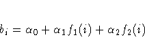
y_t = a + b₀x_t + b₁x_t-1 + b₂x_t-2 + b₃x_t-3 + b₄x_t-4 + c z_t + u_t

$b_{i} = {\alpha}_{0} + {\alpha}_{1}f_{1}(i) + {\alpha}_{2}f_{2}(i)$

where f₁(i) is a polynomial of degree 1 in i and f₂(i) is a polynomial of degree 2 in i.

Lag distribution specifications are enclosed in parentheses and follow the name of the regressor variable. The general form of the lag distribution specification is

regressor-name ( length, degree, minimum-degree, end-constraint )

where:

length: is the length of the lag distribution; that is, the number of lags of the regressor to use
degree: is the degree of the distribution polynomial
minimum-degree: is an optional minimum degree for the distribution polynomial
end-constraint: is an optional endpoint restriction specification, which can have the values FIRST, LAST, or BOTH

If the minimum-degree option is specified, the PDLREG procedure estimates models for all degrees between minimum-degree and degree.

Introductory Example

The following statements generate simulated data for variables Y and X. Y depends on the first three lags of X, with coefficients .25, .5, and .25. Thus, the effect of changes of X on Y takes effect 25% after one period, 75% after two periods, and 100% after three periods.

   data test;
      xl1 = 0; xl2 = 0; xl3 = 0;
      do t = -3 to 100;
         x = ranuni(1234);
         y = 10 + .25 * xl1 + .5 * xl2 + .25 * xl3 + .1 * rannor(1234);
         if t > 0 then output;
         xl3 = xl2; xl2 = xl1; xl1 = x;
         end;
   run;

The following statements use the PDLREG procedure to regress Y on a distributed lag of X. The length of the lag distribution is 4, and the degree of the distribution polynomial is specified as 3.

   proc pdlreg data=test;
      model y = x( 4, 3 );
   run;

The PDLREG procedure first prints a table of statistics for the residuals of the model, as shown in Figure 15.1. See Chapter 8 for an explanation of these statistics.

The PDLREG Procedure

Dependent Variable	y

Ordinary Least Squares Estimates
SSE	0.86604442	DFE	91
MSE	0.00952	Root MSE	0.09755
SBC	-156.72612	AIC	-169.54786
Regress R-Square	0.7711	Total R-Square	0.7711
Durbin-Watson	1.9920

Figure 15.1: Residual Statistics

The PDLREG procedure next prints a table of parameter estimates, standard errors, and t-tests, as shown in Figure 15.2.

The PDLREG Procedure

Variable	DF	Estimate	Standard Error	t Value	Approx Pr > \|t\|
Intercept	1	10.0030	0.0431	231.87	<.0001
x0**	1	0.4406	0.0378	11.66	<.0001
x1**	1	0.0113	0.0336	0.34	0.7377
x2**	1	-0.4108	0.0322	-12.75	<.0001
x3**	1	0.0331	0.0392	0.84	0.4007

Figure 15.2: Parameter Estimates

The preceding table shows the model intercept and the estimated parameters of the lag distribution polynomial. The parameter labeled X**0 is the constant term, ${{\alpha}_{0}}$ ,of the distribution polynomial. X**1 is the linear coefficient, ${{\alpha}_{1}}$ ,X**2 is the quadratic coefficient, ${{\alpha}_{2}}$ , and X**3 is the cubic coefficient, ${{\alpha}_{3}}$ .

The parameter estimates for the distribution polynomial are not of interest in themselves. Since the PDLREG procedure does not print the orthogonal polynomial basis that it constructs to represent the distribution polynomial, these coefficient values cannot be interpreted.

However, because these estimates are for an orthogonal basis, you can use these results to test the degree of the polynomial. For example, this table shows that the X**3 estimate is not significant; the p-value for its t ratio is .4007, while the X**2 estimate is highly significant (p<.0001). This indicates that a second-degree polynomial may be more appropriate for this data set.

The PDLREG procedure next prints the lag distribution coefficients and a graphical display of these coefficients, as shown in Figure 15.3.

The PDLREG Procedure

Estimate of Lag Distribution
Variable	Estimate	Standard Error	t Value	Approx Pr > \|t\|	-0.04 0.4167
x(0)	-0.040150	0.0360	-1.12	0.2677	\|***\| \|
x(1)	0.324241	0.0307	10.55	<.0001	\| \|***************************** \|
x(2)	0.416661	0.0239	17.45	<.0001	\| \|*************************************\|
x(3)	0.289482	0.0315	9.20	<.0001	\| \|************************** \|
x(4)	-0.004926	0.0365	-0.13	0.8929	\| \| \|

Figure 15.3: Coefficients and Graph of Estimated Lag Distribution

The lag distribution coefficients are the coefficients of the lagged values of X in the regression model. These coefficients lie on the polynomial curve defined by the parameters shown in Figure 15.2. Note that the estimated values for X(1), X(2), and X(3) are highly significant, while X(0) and X(4) are not significantly different from 0. These estimates are reasonably close to the true values used to generate the simulated data.

The graphical display of the lag distribution coefficients plots the estimated lag distribution polynomial reported in Figure 15.2. The roughly quadratic shape of this plot is another indication that a third-degree distribution curve is not needed for this data set.

Chapter Contents
Previous
Next
Top