Parks Method (Autoregressive Model)

The TSCSREG Procedure

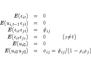
Parks Method (Autoregressive Model)

Parks (1967) considered the first-order autoregressive model in which the random errors u_it , i = 1, 2, ... , N, t = 1, 2, ... , T, have the structure

$E( u^2_{it})&=&{\sigma}_{ii} \hspace*{1.5in}\rm{(heteroscedasticity)} \cr E(u_... ... {\rho}_{i} u_{i,t-1}+ {\epsilon}_{it} \hspace*{0.9in}\rm{(autoregression)}$

where

$E( {\epsilon}_{it})&=&0 \cr E( u_{i,t-1} {\epsilon}_{jt})&=&0 \cr E( {\epsilon... ...r E( u_{i0} u_{j0})&=& {\sigma}_{ij}={\phi}_{ij}/(1- {\rho}_{i} {\rho}_{j})$

The model assumed is first-order autoregressive with contemporaneous correlation between cross sections. In this model, the covariance matrix for the vector of random errors u can be expressed as

$E( {uu}^{'})=V= [\matrix{ {\sigma}_{11}P_{11} & {\sigma}_{12}P_{12} & { ... }... ...ma}_{N1}P_{N1} & {\sigma}_{N2}P_{N2} & { ... } & {\sigma}_{NN}P_{NN} \cr } ]$

where

$P_{ij}= [\matrix{ 1 & {\rho}_{j} & {\rho}_{j}^2 & { ... } & {\rho}^{T-1}_{j} \... ...{\rho}^{T-1}_{i} & {\rho}^{T-2}_{i} & {\rho}^{T-3}_{i} & { ... } & 1 \cr } ]$

The matrix V is estimated by a two-stage procedure, and ${\beta}$ is then estimated by generalized least squares. The first step in estimating V involves the use of ordinary least squares to estimate ${\beta}$ and obtain the fitted residuals, as follows:

$\hat{u}=y-X\hat{\beta}_{OLS}$

A consistent estimator of the first-order autoregressive parameter is then obtained in the usual manner, as follows:

$\hat{\rho}_{i}= (\sum_{t=2}^T \hat{u}_{it} \hat{u}_{i,t-1}) \bigg/ (\sum_{t=2}^T{\hat{u}^2_{i,t-1}}) \hspace*{1em} i=1, 2, { ... }, N$

Finally, the autoregressive characteristic of the data can be removed (asymptotically) by the usual transformation of taking weighted differences. That is, for i = 1,2, ... ,N,

$y_{i1}\sqrt{1- \hat{\rho}^2_{i}}= \sum_{k=1}^p{X_{i1k}{{\beta}}_{k}} \sqrt{1- \hat{\rho}^2_{i}} +u_{i1}\sqrt{1- \hat{\rho}^2_{i}}$

$y_{it}- \hat{\rho}_{i} y_{i,t-1} =\sum_{k=1}^p{( X_{itk}- \hat{\rho}_{i} X_... ...}) {\beta}_{k}} + u_{it}- \hat{\rho}_{i} u_{i,t-1} \hspace*{1em}t=2,{ ... },T$

which is written

$y^{\ast}_{it}= \sum_{k=1}^p{X^{\ast}_{itk} {\beta}_{k}}+ u^{\ast}_{it} \hspace*{1em} i=1, 2, { ... }, N; \hspace*{1em} t=1, 2, { ... }, T$

Notice that the transformed model has not lost any observations (Seely and Zyskind 1971).

The second step in estimating the covariance matrix V is to apply ordinary least squares to the preceding transformed model, obtaining

$\hat{u}^{\ast}= y^{\ast}- X^{\ast} {{\beta}}^{\ast}_{OLS}$

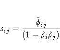
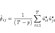
from which the consistent estimator of ${\sigma}$ _ij is calculated:

$s_{ij}=\frac{\hat{\phi}_{ij}}{(1- \hat{\rho}_{i} \hat{\rho}_{j}) }$

where

$\hat{\phi}_{ij}=\frac{1}{(T-p)} \sum_{t=1}^T \hat{u}^{\ast}_{it} \hat{u}^{\ast}_{jt}$

EGLS then proceeds in the usual manner,

$\hat{\beta}_{P}= ({X'}\hat{V}^{-1}X)^{-1} {X'}\hat{V}^{-1}y$

where $\hat{V}$ is the derived consistent estimator of V. For computational purposes, it should be pointed out that ${\hat{\beta}_{P}}$ is obtained directly from the transformed model,

$\hat{\beta}_{P}= ({X^{\ast'}}(\hat{\Phi}^{-1}{\otimes}I_{T}) X^{\ast})^{-1}{X^{\ast'}} (\hat{\Phi}^{-1}{\otimes}I_{T}) y^{\ast}$

where ${\hat{\Phi}= [\hat{\phi}_{ij}]_{i,j=1,{ ... },N} }$ .

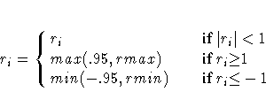
The preceding procedure is equivalent to Zellner's two-stage methodology applied to the transformed model (Zellner 1962). Parks demonstrates that his estimator is consistent and asymptotically, normally distributed with

$\rm{Var}(\hat{\beta}_{P})= ({X'}V^{-1}X)^{-1}$

Standard Corrections

For the PARKS option, the first-order autocorrelation coefficient must be estimated for each cross section. Let ${\rho}$ be the N*1 vector of true parameters and R = (r₁, ... ,r_N)' be the corresponding vector of estimates. Then, to ensure that only range-preserving estimates are used in PROC TSCSREG, the following modification for R is made:

$r_{i} = \cases{ r_{i} &\hspace*{1em}\rm{if} {| r_{i}|}\lt 1\space \cr max(.9... ...}1\space \cr min(-.95, rmin) &\hspace*{1em}\rm{if} r_{i}{\le}-1\space \cr }$

where

$rmax = \cases{ 0 & \hspace*{1em}\rm{if} r_{i} \lt 0\space \rm{or} r_{i}{\ge}1 ... ...s_{j} [ r_{j} : 0 {\le} r_{j} \lt 1 ] & \hspace*{1em}\rm{otherwise} \cr }$

and

$rmin = \cases{ 0 & \hspace*{1em}\rm{if} r_{i} \gt 0\space \rm{or} r_{i}{\le}-1... ...s_{j} [ r_{j} : -1 \lt r_{j} {\le} 0 ] &\hspace*{1em}\rm{otherwise} \cr }$

Whenever this correction is made, a warning message is printed.

Chapter Contents
Previous
Next
Top