Details of Model Selection

The X11 Procedure

Details of Model Selection

If an ARIMA statement is present, but no MODEL= is given, PROC X11 estimates and forecasts five predefined models and selects the best. This section describes the details of the selection criteria and the selection process.

The five predefined models used by PROC X11 are the same as those used by X11ARIMA/88 from Statistics Canada. These particular models, shown in Table 21.1 were chosen on the basis of testing a large number of economics series (Dagum, 1988) and should provide reasonable forecasts for most economic series.

Table 21.1: Five Predefined Models

Model #	Specification	Multiplicative	Additive
1	(0,1,1)(0,1,1)s	log transform	no transform
2	(0,1,2)(0,1,1)s	log transform	no transform
3	(2,1,0)(0,1,1)s	log transform	no transform
4	(0,2,2)(0,1,1)s	log transform	no transform
5	(2,1,2)(0,1,1)s	no transform	no transform

The selection process proceeds as follows. The five models are estimated and one-step-ahead forecasts are produced in the order shown in Table 21.1. As each model is estimated the following three criteria are checked:

The Mean Absolute Percent Error (MAPE) for the last three years of the series must be less than 15 %.
The significance probability for the Box-Ljung Chi-square for up to lag 24 for monthly (8 for quarterly) must greater than 0.05.
The over-differencing criteria must not exceed 0.9.

The description of these three criteria are given in "Criteria Details." The default values for these criteria are those used by X11ARIMA/88 from Statistics Canada; these defaults can be changed by the MAPECR=, CHICR= and OVDIFCR= options.

A model that fails any one of these three criteria is excluded from further consideration. In addition, if the ARIMA estimation fails for a given model, a warning is issued, and the model is excluded. The final set of all models considered are those that pass all three criteria and are estimated successfully. From this set, the model with the smallest MAPE for the last three years is chosen.

If all five models fail, ARIMA processing is skipped for the variable being processed, and the standard X-11 seasonal adjustment is performed. A note is written to the log with this information.

The chosen model is then used to forecast the series one or more years (determined by the FORECAST= option on the ARIMA statement). These forecasts are appended on the original data (or the prior and calendar-adjusted data).

If a BACKCAST= is specified, the chosen model form is used, but the parameters are reestimated using the reversed series. Using these parameters, the reversed series is forecasted for the number of years specified by the BACKCAST= option. These forecasts are then reversed and appended to the beginning of the original series, or the prior and calendar-adjusted series, to produce the backcasts.

Note that the final selection rule (the smallest MAPE using the last three years) emphasizes the quality of the forecasts at the end of the series. This is consistent with the purpose of the X-11-ARIMA methodology, namely, to improve the estimates of seasonal factors and thus minimize revisions to recent past data as new data become available.

Criteria Details

The Mean Absolute Percent Error (MAPE)

For the MAPE criteria testing, only the last three years of the original series (or prior and calendar adjusted series) is used in computing the MAPE.

Let y_t, t=1,..,n be the last three years of the series, and denote its one-step-ahead forecast by ${\hat{y}_{t}}$ , where n=36 for a monthly series, and n=12 for a quarterly series.

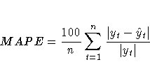
With this notation, the MAPE criteria is computed as

$MAPE = \frac{100}n\sum_{t=1}^n{\frac{{| y_{t}-\hat{y}_{t}|}}{{| y_{t}|} }}$

Box-Ljung Chi-Square

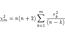
The Box-Ljung Chi-Square is a lack of fit test using the model residuals. This test statistic is computed using the Ljung-Box formula

${\chi}^2_{m} =n(n+2)\sum_{k=1}^m{\frac{r^2_{k}}{(n-k) } }$

where n is the number of residuals that can be computed for the time series, and

$r_{k}=\frac{\sum_{t=1}^{n-k}{a_{t} a_{t+k}}}{\sum_{t=1}^n{a^2_{t}} }$

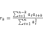
where the a_t's are the residual sequence. This formula has been suggested by Ljung and Box as yielding a better fit to the asymptotic chi-square distribution. Some simulation studies of the finite sample properties of this statistic are given by Davies, Triggs, and Newbold (1977) and by Ljung and Box (1978).

For monthly series, m=24, while for quarterly series, m=8.

Over-Differencing Test

From Table 21.1 you can se that all models have a single seasonal MA factor and at most two nonseasonal MA factors. Also, all models have seasonal and nonseasonal differencing. Consider model 2 applied to a monthly series y_t with ${E(y_{t}) = {\mu}}$ :

$(1-B^1)(1-B^{12})(y_{t} - {\mu}) = (1-{\theta}_{1}B- {\theta}_{2}B^2) (1-{\theta}_{3}B^{12})a_{t}$

If ${{\theta}_{3} = 1.0}$ , then the factors ${(1-{\theta}_{3}B^{12})}$ and (1-B¹²) will cancel, resulting in a lower-order model.

Similarly, if ${{\theta}_{1}+{\theta}_{2} = 1.0}$ ,

$(1-{\theta}_{1}B- {\theta}_{2}B^2) = (1-B)(1-{\alpha}B)$

for some ${{\alpha}{\neq}0.0}$ . Again, this results in cancellation and a lower order model.

Since the parameters are not exact, it is not reasonable to require that

${\theta}_{3} \lt 1.0 {\rm and} {\theta}_{1}+{\theta}_{2} \lt 1.0$

Instead, an approximate test is performed by requiring that

${\theta}_{3} {\leq} 0.9 {\rm and} {\theta}_{1}+{\theta}_{2} {\leq} 0.9$

The default value of 0.9 can be changed by the OVDIFCR= option. Similar reasoning applies to the other models.

ARIMA Statement Options for the Five Predefined Models

The following table lists the five predefined models and gives the equivalent MODEL= parameters in a PROC X11 ARIMA statement.

In all models except the fifth, a log transformation is performed before the ARIMA estimation for the multiplicative case; no transformation is performed for the additive case. For the fifth model, no transformation is done for either case.

The multiplicative case is assumed in the following table. The indicated seasonality s in the specification is either 12 (monthly), or 4 (quarterly). The MODEL statement assumes a monthly series.

Table 21.2: ARIMA Statements Options for Predefined Models

Model	ARIMA Statement Options
(0,1,1)(0,1,1)s	MODEL=( Q=1 SQ=1 DIF=1 SDIF=1 ) TRANSFORM=LOG
(0,1,2)(0,1,1)s	MODEL=( Q=2 SQ=1 DIF=1 SDIF=1 ) TRANSFORM=LOG
(2,1,0)(0,1,1)s	MODEL=( P=2 SQ=1 DIF=1 SDIF=1 ) TRANSFORM=LOG
(0,2,2)(0,1,1)s	MODEL=( Q=2 SQ=1 DIF=2 SDIF=1 ) TRANSFORM=LOG
(2,1,2)(0,1,1)s	MODEL=( P=2 Q=2 SQ=1 DIF=1 SDIF=1 )

Chapter Contents
Previous
Next
Top