Analysis of Variance

Creating the Analysis of Variance

Consider the two-way analysis of variance model Kutner (1974) proposed for these data: ${ {CHANG\_BP}_{ijk} = {\mu} + {\gamma}_{i} + {\tau}_{j} + ({\gamma}{\tau})_{ij} + {\epsilon}_{ijk}}$

where ${\mu}$ is the overall mean effect, ${ {\gamma}_{i}}$ is the effect of the ith level of DRUG, ${ {\tau}_{j}}$ is the effect of the jth level of DISEASE, ${ ({\gamma}{\tau})_{ij}}$ is the joint effect of the ith level of DRUG with the jth level of DISEASE, and ${ {\epsilon}_{ijk}}$ is the random error term for the kth observation in the ith level of DRUG and jth level of DISEASE. The ${ {\epsilon}_{ijk}}$ 's are assumed to be normally distributed and uncorrelated and to have mean 0 and common variance ${ {\sigma}^2}$ .

The effects for DRUG and DISEASE are often referred to as the main effects in the model and the DRUG*DISEASE effect as an interaction effect. The interaction effect enables you to determine whether the level of DRUG affects the change in blood pressure differently for different levels of DISEASE. To begin the analysis of variance, follow these steps.

Choose Analyze:Fit (Y X).

Select CHANG_BP in the variables list on the left, then click the Y button.

CHANG_BP appears in the Y variables list and is now defined as the response variable.

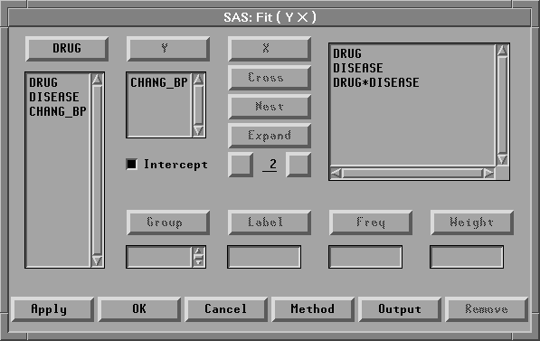
Select DRUG and DISEASE, then click the Expand button.

Your variables dialog should now appear, as shown in Figure 15.5.

Figure 15.5: Fit Variables Dialog with Variable Roles Assigned

The Expand button provides a convenient way to specify interactions of any order. The degree of expansion is controlled by the value below the Expand button. The order 2 is the default, so clicking Expand constructs all possible effects from the selected variables up to second-order effects. This adds DRUG, DISEASE, and DRUG*DISEASE to the effects list.

Note You could have added the same effects by using the X and Cross buttons, but the Expand button is faster. There is also a Nest button for specifying nested effects. For more information on the effects buttons, see Chapter 39, "Fit Analyses."

Click the OK button.

A fit window appears, as shown in Figure 15.6.

You can control which tables and graphs the fit window contains by clicking the Output button in the fit variables dialog or by choosing from the Tables and Graphs menus. By default, the fit window contains tables for model specification, Nominal Variable Information, Parameter Information, Model Equation, Summary of Fit, Analysis of Variance, Type III Tests, and Parameter Estimates, as well as a residual-by-predicted plot.

Figure 15.6: Fit Window - Model Information

Creating the Analysis of Variance

Model Information

Summary of Fit

Analysis of Variance

Type III Tests

Parameter Estimates

Residuals-by-Predicted Plot