Model Formats: PROC LP and PROC NETFLOW

Introduction to Optimization

Model Formats: PROC LP and PROC NETFLOW

Model generation and maintainence are often difficult and expensive aspects of applying mathematical programming techniques. The flexible input formats for the optimization procedures in SAS/OR software simplify this task.

A small product mix problem serves as a starting point for a discussion of different types of model formats supported in SAS/OR software.

A candy manufacturer makes two products: chocolates and toffee. What combination of chocolates and toffee should be produced in a day in order to maximize the company's profit? Chocolates contribute $0.25 per pound to profit and toffee contributes $0.75 per pound. The variables chocolates and toffee are the decision variables.

Four processes are used to manufacture the candy:

Process 1 combines and cooks the basic ingredients for both chocolates and toffee.
Process 2 adds colors and flavors to the toffee, then cools and shapes the confection.
Process 3 chops and mixes nuts and raisins, adds them to the chocolates, then cools and cuts the bars.
Process 4 is packaging: chocolates are placed in individual paper shells; toffee are wrapped in cellophane packages.

During the day, there are 7.5 hours (27,000 seconds) available for each process.

Firm time standards have been established for each process. For Process 1, mixing and cooking take 15 seconds for each pound of chocolate and 40 seconds for each pound of toffee. Process 2 takes 56.25 seconds per pound of toffee. For Process 3, 18.75 seconds are required for each pound of chocolate. In packaging, a pound of chocolates can be wrapped in 12 seconds, whereas 50 seconds are required for a pound of toffee. These data are summarized below:

                      Available       Required per Pound
                        Time         chocolates     toffee
     Process            (sec)          (sec)         (sec)
   1 Cooking            27,000           15          40
   2 Color/Flavor       27,000                      56.25
   3 Condiments         27,000          18.75
   4 Packaging          27,000          126          50

The object is to

Maximize:: 0.25(chocolates) + 0.75(toffee)

which is the company's total profit.

The production of the candy is limited by the time available for each process. The limits placed on production by Process 1 are expressed by the inequality

Process 1:: $15(chocolates) + 40(toffee) \leq 27,000$

Process 1 can handle any combination of chocolates and toffee that satisfies this inequality.

The limits on production by other processes generate constraints described by these inequalities:

Process 2:: $56.25(toffee) \leq 27,000$
Process 3:: $18.75(chocolates) \leq 27,000$
Process 4:: $12(chocolates) + 50(toffee) \leq 27,000$

This linear program illustrates the type of problem known as a product mix example. The mix of products that maximizes the objective without violating the constraints is the solution. There are two formats that can represent this model.

Dense format

The following DATA step creates a SAS data set for the preceding problem. Notice that the values of CHOCO and TOFFEE in the data set are the coefficients of those variables in the equations corresponding to the objective function and constraints. The variable _id_ contains a character string that names the rows in the problem data set. The variable _type_ is a character variable that contains keywords that describes the type of each row in the problem data set. And the variable _rhs_ contains the right-hand-side values.

   data factory;
      input _id_ $ CHOCO TOFFEE _type_ $ _rhs_;
      datalines;
object      0.25    0.75   MAX     .
process1   15.00   40.00   LE  27000
process2    0.00   56.25   LE  27000
process3   18.75    0.00   LE  27000
process4   12.00   50.00   LE  27000
   ;

To solve this using the Interior Point algorithm of PROC NETFLOW, specify:

   proc netflow arcdata=factory condata=factory;

However, this example will be solved by the LP procedure. Because the special variables _id_, _type_, and _rhs_ are used in the problem data set, there is no need to identify them to the LP procedure.

   proc lp;

The output from the LP procedure is in four sections.

Problem Summary

The first section of the output, PROBLEM SUMMARY, describes the problem by identifying the objective function (defined by the first observation in the data set used as input); the right-hand-side variable; the type variable; and the density of the problem. The problem density describes the relative number of elements in the problem matrix that are nonzero. The fewer zeros in the matrix, the higher the problem density. The PROBLEM SUMMARY describes the problem giving the number and type of variables in the model and the number and type of constraints. The types of variables in the problem are identified. Variables are either structural or logical. Structural variables are identified in the VAR statement, when the dense format is used. They are the unknowns in the equations defining the objective function and constraints. By default, PROC LP assumes that structural variables have the additional constraint that they must be nonnegative. Upper and lower bounds to structural variables can be defined.

The SAS System

The LP Procedure

Problem Summary
Objective Function	Max object
Rhs Variable	_rhs_
Type Variable	_type_
Problem Density (%)	41.67

Variables	Number

Non-negative	2
Slack	4

Total	6

Constraints	Number

LE	4
Objective	1

Total	5

Figure 1.8: PROBLEM SUMMARY

The Problem Summary shows, for example, that there are 2 nonnegative decision variables, namely CHOCO and TOFFEE. It also shows that there are 4 constraints of type LE.

After the procedure displays this information, it solves the problem, then produces the SOLUTION SUMMARY.

Solution Summary

This section (Figure 1.9) gives information about the solution that was found; whether the optimizer terminated successfully having found the optimum.

When PROC LP solves a problem, an iterative process is used. First, the procedure finds a feasible solution, one that satisfies the constraints. The second phase finds the optimum solution from the set of feasible solutions. The SOLUTION SUMMARY gives the number of iterations the procedure took in each of these phases, the number of variables in the initial feasible solution, the time the procedure used to solve the problem, and the number of matrix inversions necessary.

The LP Procedure

Solution Summary
Terminated Successfully
Objective Value	475

Phase 1 Iterations	0
Phase 2 Iterations	3
Phase 3 Iterations	0
Integer Iterations	0
Integer Solutions	0
Initial Basic Feasible Variables	6
Time Used (seconds)	0
Number of Inversions	2

Epsilon	1E-8
Infinity	1.797693E308
Maximum Phase 1 Iterations	100
Maximum Phase 2 Iterations	100
Maximum Phase 3 Iterations	99999999
Maximum Integer Iterations	100
Time Limit (seconds)	120

Figure 1.9: SOLUTION SUMMARY

After performing 3 phase 2 iterations, the procedure terminated successfully finding an optimum with optimal objective value of 475.

Variable Summary

The next section of the output is the VARIABLE SUMMARY. For each variable, the variable summary (Figure 1.10) gives the value, objective function coefficient, status in the solution, and reduced cost.

The LP Procedure

Variable Summary
Col	Variable Name	Status	Type	Price	Activity	Reduced Cost
1	CHOCO	BASIC	NON-NEG	0.25	1000	0
2	TOFFEE	BASIC	NON-NEG	0.75	300	0
3	process1		SLACK	0	0	-0.012963
4	process2	BASIC	SLACK	0	10125	0
5	process3	BASIC	SLACK	0	8250	0
6	process4		SLACK	0	0	-0.00463

Figure 1.10: VARIABLE SUMMARY

The VARIABLE SUMMARY contains details about each variable in the solution. The Activity column shows that optimum profitability is achieved when 1000 pounds of chocolate and 300 pounds of toffee are produced. The variables process1, process2, process3, and process4 correspond to the four slack variables in the Process 1, Process 2, Process 3, and Process 4 constraints, respectively. Producing 1000 pounds of chocolate and 300 pounds of toffee a day leaves 10,125 seconds of slack time in Process 2 (where colors and flavors are added to the toffee) and 8,250 seconds of slack time in Process 3 (where nuts and raisins are mixed and added to the chocolate).

Constraint Summary

The last section of the output is the CONSTRAINT SUMMARY. This output (Figure 1.11) gives the value of the objective function, the value of each constraint, and the dual activities.

The ACTIVITY column gives the value of the right-hand side of each equation when the problem is solved using the information given in the previous table.

The DUAL ACTIVITY column reveals that each second in Process 1 (mixing-cooking) is worth approximately $.013, and each second in Process 4 (Packaging), is worth approximately $.005. These figures (called shadow prices) can be used to decide whether the total available time for Processes 1 and 4 should be increased. If a second can be added to the total production time in Processes 1 for less than $.013, it would be profitable to do so. The dual activities for Process 1 and 4 are zero since adding time to those processes does not increase profits. Keep in mind that the dual activity gives the marginal improvement to the objective and that adding time to Process 1 changes the original problem and solution.

The LP Procedure

Constraint Summary
Row	Constraint Name	Type	S/S Col	Rhs	Activity	Dual Activity
1	object	OBJECTVE	.	0	475	.
2	process1	LE	3	27000	27000	0.012963
3	process2	LE	4	27000	16875	0
4	process3	LE	5	27000	18750	0
5	process4	LE	6	27000	27000	0.0046296

Figure 1.11: CONSTRAINT SUMMARY

For a complete description of the output from PROC LP, see the chapter on teh LP procedure.

Sparse Format

Typically, mathematical programming models are sparse. That is, few of the coefficients in the constraint matrix are nonzero. The dense problem format shown in the last section would be an inefficient way to represent sparse models. The LP procedure also accepts data in a sparse input format. Only the nonzero coefficients need be specified. It is consistent with the standard MPS sparse format and much more flexible so that models using the MPS format can be easily converted to the LP format. The appendix at the end of this book describes a SAS macro for conversion.

Although the factory example of the last section is not sparse, illustrated here is an example of the sparse input format. The sparse data set has four variables: a row type identifying variable, a row name variable, a column name variable, and a coefficient variable.

   data factory;
      format _type_ $8. _row_ $16. _col_ $16.;
      input _type_ $_row_ $ _col_ $ _coef_ ;
      datalines;        
max      object     .            .
.        object     chocolate    .25
.        object     toffee       .75
le       process1   .            .
.        process1   chocolate    15
.        process1   toffee       40
.        process1   _RHS_        27000
le       process2   .            .
.        process2   toffee       56.25
.        process2   _RHS_        27000
le       process3   .            .
.        process3   chocolate    18.75
.        process3   _RHS_        27000
le       process4   .            .
.        process4   chocolate    12
.        process4   toffee       50
.        process4   _RHS_        27000
   ;

To solve this problem using the Interior Point algorithm of PROC NETFLOW, specify

   proc netflow sparsecondata arcdata=factory condata=factory;

However, this example will be solved by the LP procedure.

Notice that the _type_ variable contains keywords as for the dense format, the _row_ variable contains the row names in the model, the _col_ variable contains the column names in the model, and the _coef_ variable contains the coefficients for that particular row and column. Since the row and column names are the values of variables in a SAS data set, they are not limited to 8 characters. This feature, as well as the order independence of the format, simplify matrix generation.

The SPARSEDATA option in the PROC LP statement tells the LP procedure that the model in the problem data set is in the sparse format. This example also illustrates how the solution of the linear program is saved in two output data sets: the primal data set and the dual data set.

   proc lp 
      data=factory sparsedata 
      primalout=primal dualout=dual;
   run;

The primal data set (Figure 1.12) contains the information that is displayed in the VARIABLE SUMMARY plus additional information about the bounds on the variables.

Obs	_OBJ_ID_	_RHS_ID_	_VAR_	_TYPE_	_STATUS_	_LBOUND_	_VALUE_	_UBOUND_	_PRICE_	_R_COST_
1	object	_RHS_	chocolate	NON-NEG	_BASIC_	0	1000	1.7977E308	0.25	-0.000000
2	object	_RHS_	toffee	NON-NEG	_BASIC_	0	300	1.7977E308	0.75	0.000000
3	object	_RHS_	process1	SLACK		0	0	1.7977E308	0.00	-0.012963
4	object	_RHS_	process2	SLACK	_BASIC_	0	10125	1.7977E308	0.00	0.000000
5	object	_RHS_	process3	SLACK	_BASIC_	0	8250	1.7977E308	0.00	0.000000
6	object	_RHS_	process4	SLACK		0	0	1.7977E308	0.00	-0.004630
7	object	_RHS_	PHASE_1_OBJECTIV	OBJECT	_DEGEN_	0	0	0	0.00	0.000000
8	object	_RHS_	object	OBJECT	_BASIC_	0	475	1.7977E308	0.00	0.000000

Figure 1.12: Primal data set

The dual data set (Figure 1.13) contains the information that is displayed in the CONSTRAINT SUMMARY plus additional information about bounds on the rows.

Obs	_OBJ_ID_	_RHS_ID_	_ROW_ID_	_TYPE_	_RHS_	_L_RHS_	_VALUE_	_U_RHS_	_DUAL_
1	object	_RHS_	object	OBJECT	475	475	475	475	.
2	object	_RHS_	process1	LE	27000	-1.7977E308	27000	27000	0.012963
3	object	_RHS_	process2	LE	27000	-1.7977E308	16875	27000	0.000000
4	object	_RHS_	process3	LE	27000	-1.7977E308	18750	27000	0.000000
5	object	_RHS_	process4	LE	27000	-1.7977E308	27000	27000	0.004630

Figure 1.13: Dual data set

Network Format

Network flow problems can be described by specifing the nodes in the network and their supplies and demands, and the arcs in the network and their costs and capacities and lower flow bounds. Consider the simple transshipment problem in Figure 1.14 as an illustration.

Figure 1.14: Transshipment Problem

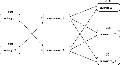
Suppose the candy manufacturing company has two factories, two warehouses, and three customers for chocolate. The two factories each have a production capacity of 500 pounds per day. The three customers have demands of 100, 200, and 50 pounds per day, respectively.

The following data set describes the supplies (positive values for the supdem variable) and the demands (negative values for the supdem variable) for each of the customers and factories.

   data nodes;
      format node $16. ;
      input node $ supdem;
      datalines;
customer_1   -100
customer_2   -200
customer_3    -50
factory_1     500
factory_2     500
   ;

Suppose that there are two warehouses that are used to store the chocolate before shipment to the customers and that there are different costs for shipping between each factory, warehouse, and customer.

What is the minimum cost routing for supplying the customers?

Arcs are described in another data set. Each observation defines a new arc in the network and gives data about the arc. For example, there is an arc between the node factory_1 and the node warehouse_1. Each unit of flow on that arc costs 10. Although this example does not include it, lower and upper bounds on the flow across that arc can be listed here.

   data network;
      format from $16. to $16.;
      input from $ to $ cost ;
      datalines;
factory_1     warehouse_1  10 
factory_2     warehouse_1   5
factory_1     warehouse_2   7
factory_2     warehouse_2   9
warehouse_1   customer_1    3
warehouse_1   customer_2    4
warehouse_1   customer_3    4
warehouse_2   customer_1    5
warehouse_2   customer_2    5
warehouse_2   customer_3    6
   ;

Use PROC NETFLOW to find the minimum cost routing. This procedure takes the model as defined in the network and nodes data sets and finds the minimum cost flow.

   proc netflow arcout=arc_sav
                arcdata=network nodedata=nodes;
     node node;      /* node data set information */
     supdem supdem;
 
     tail from;      /* arc data set information */
     head to; 
     cost cost;

     run;

   proc print;
      var from to cost _capac_ _lo_ _supply_ _demand_  
          _flow_ _fcost_ _rcost_;
      sum _fcost_;
      run;

PROC NETFLOW produces the following on the SAS log:

NOTE: Number of nodes= 7 .
NOTE: Number of supply nodes= 2 .
NOTE: Number of demand nodes= 3 .
NOTE: Total supply= 1000 , total demand= 350 .
NOTE: Number of arcs= 10 .
NOTE: Number of iterations performed (neglecting any constraints)= 7 .
NOTE: Of these, 2 were degenerate.
NOTE: Optimum (neglecting any constraints) found.
NOTE: Minimal total cost= 3050 .
NOTE: The data set WORK.ARC_SAV has 10 observations and 13 variables.

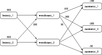
The solution (Figure 1.15) saved in the arc_sav data set shows the optimal amount of chocolate to send across each arc (the amount to ship from each factory to each warehouse and from each warehouse to each customer) in the network per day.

Obs	from	to	cost	_CAPAC_	_LO_	_SUPPLY_	_DEMAND_	_FLOW_	_FCOST_	_RCOST_
1	warehouse_1	customer_1	3	99999999	0	.	100	100	300	.
2	warehouse_2	customer_1	5	99999999	0	.	100	0	0	4
3	warehouse_1	customer_2	4	99999999	0	.	200	200	800	.
4	warehouse_2	customer_2	5	99999999	0	.	200	0	0	3
5	warehouse_1	customer_3	4	99999999	0	.	50	50	200	.
6	warehouse_2	customer_3	6	99999999	0	.	50	0	0	4
7	factory_1	warehouse_1	10	99999999	0	500	.	0	0	5
8	factory_2	warehouse_1	5	99999999	0	500	.	350	1750	.
9	factory_1	warehouse_2	7	99999999	0	500	.	0	0	.
10	factory_2	warehouse_2	9	99999999	0	500	.	0	0	2
									3050

Figure 1.15: ARCOUT data set

Notice which arcs have positive flow (_FLOW_ is greater than 0). These arcs indicate the amount of chocolate that should be sent from factory_2 to warehouse_1 and from there on to the three customers. The model indicates no production at factory_1 and no use of warehouse_2.

Figure 1.16: Optimal Solution for the Transshipment Problem

Chapter Contents
Previous
Next
Top